Next: Adjointness and ordinary differential
Up: PHASE-SHIFT MIGRATION
Previous: Kirchhoff versus phase-shift migration
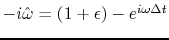
The definition of  as
as
 obscures two aspects of .
First, which of the two square roots is intended,
and second, what happens when
obscures two aspects of .
First, which of the two square roots is intended,
and second, what happens when
 .
For both coding and theoretical work we
need a definition of
.
For both coding and theoretical work we
need a definition of  that is valid
for both positive and negative values of
that is valid
for both positive and negative values of  and for all
  .
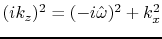
Define a function
.
Define a function
 by
by
 |
(17) |
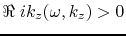
It is important to know that for any  ,
and any real and real that
the real part
,
and any real and real that
the real part  is positive.
This means we can extrapolate waves safely
with
is positive.
This means we can extrapolate waves safely
with  for increasing
  or
with
or
with  for decreasing .
To switch from downgoing to upcoming we use
the complex conjugate
for decreasing .
To switch from downgoing to upcoming we use
the complex conjugate  .
Thus we have disentangled the damping from the direction of propagation.
.
Thus we have disentangled the damping from the direction of propagation.
Let us see why is positive
for all real values of and .
Recall that for ranging between  ,
,
 rotates around the unit circle
in the complex plane.
Examine Figure 7.10
which shows the complex functions:
rotates around the unit circle
in the complex plane.
Examine Figure 7.10
which shows the complex functions:
-
 ,
,
-
 ,
,
-
 ,
,
-
 , and
, and
-
![$ik_z = [(-i \hat\omega)^2+k_x^2]^{1/2}$](img117.png)

|
|---|
francis
Figure 10.
Some functions in the complex plane.
|
|---|
![[pdf]](icons/pdf.png) ![[png]](icons/viewmag.png) ![[scons]](icons/configure.png)
|
|---|
The first two panels are explained by the first two functions.
The first two functions and the first two panels look different
but they become the same in the practical limit
of
 and
and
 .
The left panel represents a time derivative in continuous time,
and the second panel likewise
in sampled time is for
a ``causal finite-difference operator''
representing a time derivative.
Notice that the graphs look the same near
.
The left panel represents a time derivative in continuous time,
and the second panel likewise
in sampled time is for
a ``causal finite-difference operator''
representing a time derivative.
Notice that the graphs look the same near  .
As we sample seismic data with increasing density,
,
the frequency content shifts further away from the Nyquist frequency.
Measuring in radians/sample,
in the limit
, the physical energy is all near
.
.
As we sample seismic data with increasing density,
,
the frequency content shifts further away from the Nyquist frequency.
Measuring in radians/sample,
in the limit
, the physical energy is all near
.
The third panel in Figure 7.10
shows
which is a cardioid that
wraps itself close up to the negative imaginary axis without touching it.
(To understand the shape near the origin, think about the square
of the leftmost plane. You may have seen examples
of the negative imaginary axis being a branch cut.)
In the fourth panel a small positive quantity  is added which
shifts the cardioid to the right a bit.
Taking the square root gives the last panel
which shows the curve in the right half plane
thus proving
the important result we need,
that
is added which
shifts the cardioid to the right a bit.
Taking the square root gives the last panel
which shows the curve in the right half plane
thus proving
the important result we need,
that
 for all real .
It is also positive for all real because
any
for all real .
It is also positive for all real because
any  shifts the cardioid to the right.
The additional issue of time causality in forward modeling
is covered in IEI.
shifts the cardioid to the right.
The additional issue of time causality in forward modeling
is covered in IEI.
Finally, you might ask, why bother with all this careful theory
connected with the damped square root.
Why not simply abandon the evanescent waves?
There are several reasons:
- The exploding reflector concept fails for evanescent waves
(when
 ).
Realistic modeling would have them damping with depth.
Rather than trying to handle them correctly we will make a choice,
either (1) to abandon evanescent waves effectively setting them to zero,
or (2) we will take them to be damping.
(You might notice that when we switch from downgoing to upgoing,
a damping exponential switches to a growing exponential,
but when we consider the adjoint of applying a damped exponential,
that adjoint is also a damped exponential.)
).
Realistic modeling would have them damping with depth.
Rather than trying to handle them correctly we will make a choice,
either (1) to abandon evanescent waves effectively setting them to zero,
or (2) we will take them to be damping.
(You might notice that when we switch from downgoing to upgoing,
a damping exponential switches to a growing exponential,
but when we consider the adjoint of applying a damped exponential,
that adjoint is also a damped exponential.)
I'm not sure if there is a practical difference between
choosing to damp evanescent waves or simply to set them to zero,
but there should be a noticable difference on synthetic data:
When a Fourier-domain amplitude drops abruptly
from unity to zero, we can expect a time-domain signal
that spreads widely on the time axis,
perhaps dropping off slowly as  .
We can expect a more concentrated pulse
if we include the evanescent energy, even though it is small.
I predict the following behavior:
Take an impulse; diffract it and then migrate it.
When evanescent waves have been truncated, I predict
the impulse is turned into a ``butterfly'' whose wings
are at the hyperbola asymptote.
Damping the evanescent waves, I predict,
gives us more of a ``rounded'' impulse.
.
We can expect a more concentrated pulse
if we include the evanescent energy, even though it is small.
I predict the following behavior:
Take an impulse; diffract it and then migrate it.
When evanescent waves have been truncated, I predict
the impulse is turned into a ``butterfly'' whose wings
are at the hyperbola asymptote.
Damping the evanescent waves, I predict,
gives us more of a ``rounded'' impulse.
- In a later chapter we will handle the
 -axis by finite differencing
(so that we can handle
-axis by finite differencing
(so that we can handle  .
There a stability problem will develop unless we begin
from careful definitions as we are doing here.
.
There a stability problem will develop unless we begin
from careful definitions as we are doing here.
- Seismic theory includes an abstract mathematical concept
known as branch-line integrals.
Such theory is most easily understood beginning from here.
Next: Adjointness and ordinary differential
Up: PHASE-SHIFT MIGRATION
Previous: Kirchhoff versus phase-shift migration
2009-03-16