|
 |
 |
 | Nonhyperbolic reflection moveout of  -waves:
An overview and comparison of reasons -waves:
An overview and comparison of reasons |  |
![[pdf]](icons/pdf.png) |
Next: CURVILINEAR REFLECTOR
Up: VERTICAL HETEROGENEITY
Previous: Vertically heterogeneous isotropic model
In a model that includes vertical heterogeneity and anisotropy, both
factors influence bending of the rays. The weak anisotropy
approximation, however, allows us to neglect the effect of anisotropy on ray
trajectories and consider its influence on traveltimes only. This
assumption is analogous to the linearization, conventionally done for
tomographic inversion. Its application to weak anisotropy has been
discussed by Grechka and McMechan (1996). According to the
linearization assumption, we can retain isotropic equation
(20) describing the ray trajectories and rewrite equation
(19) in the form
 |
(40) |
where  is the anisotropic group velocity, which varies both with the
depth
is the anisotropic group velocity, which varies both with the
depth  and with the ray angle
  and has the expression
(1). Differentiation of the parametric traveltime equations
(40) and (20) and linearization with respect to Thomsen's
anisotropic parameters shows that the general form of equations
(23)-(26) remains valid if we replace the definitions
of the root-mean-square velocity
and has the expression
(1). Differentiation of the parametric traveltime equations
(40) and (20) and linearization with respect to Thomsen's
anisotropic parameters shows that the general form of equations
(23)-(26) remains valid if we replace the definitions
of the root-mean-square velocity  and the parameters
  by
by
In homogeneous media, expressions (41)
and (42) transform series (22) with
coefficients (23)-(26) into the form equivalent to
series (13). Two important conclusions follow from
equations (41) and (42).
First, if the mean value of the anisotropic coefficient  is less than zero, the presence of anisotropy can reduce the difference
between the effective root-mean-square velocity and the effective vertical
velocity
is less than zero, the presence of anisotropy can reduce the difference
between the effective root-mean-square velocity and the effective vertical
velocity
 . In this case, the influence of anisotropy
and heterogeneity partially cancel each other, and the moveout curve
may behave at small offsets as if the medium were homogeneous and
isotropic. This behavior has been noticed by
Larner and Cohen (1993). On the other hand, if the anellipticity
coefficient
. In this case, the influence of anisotropy
and heterogeneity partially cancel each other, and the moveout curve
may behave at small offsets as if the medium were homogeneous and
isotropic. This behavior has been noticed by
Larner and Cohen (1993). On the other hand, if the anellipticity
coefficient  is positive and different from zero, it can
significantly increase the values of the heterogeneity parameters
is positive and different from zero, it can
significantly increase the values of the heterogeneity parameters
 defined by equations (29). Then, the nonhyperbolicity
of reflection moveouts at
large offsets is stronger than that in isotropic media.
defined by equations (29). Then, the nonhyperbolicity
of reflection moveouts at
large offsets is stronger than that in isotropic media.
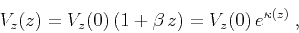
To exemplify the general theory, let us consider a simple analytic
model with constant anisotropic parameters and the vertical velocity
linearly increasing with depth according to the equation
 |
(43) |
where  is the logarithm of the velocity change. In this case,
the analytic expression for the RMS velocity is found
from equation (41) to be
is the logarithm of the velocity change. In this case,
the analytic expression for the RMS velocity is found
from equation (41) to be
 |
(44) |
while the mean vertical velocity is
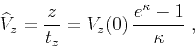 |
(45) |
where
 is evaluated at the reflector depth.
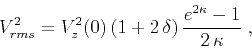
Comparing equations (44) and (45), we can see
that the squared RMS velocity
is evaluated at the reflector depth.
Comparing equations (44) and (45), we can see
that the squared RMS velocity  equals to the squared mean velocity
 if
if
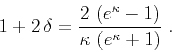 |
(46) |
For small , the estimate of from equation
(46) is
 |
(47) |
For example, if the vertical velocity near the reflector is twice
that at the surface (i.e.,
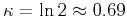 ),
having the anisotropic
parameter as small as
),
having the anisotropic
parameter as small as  is sufficient to cancel out the
influence of heterogeneity on the normal-moveout velocity. The values of
parameters
is sufficient to cancel out the
influence of heterogeneity on the normal-moveout velocity. The values of
parameters  and
and  , found from equations (29), (41) and (42), are
Substituting equations (48) and (49) into
the estimates (32) and (38) and linearizing
them both in and in , we
find that the error of anisotropic traveltime approximation
(12) in the linear velocity model is
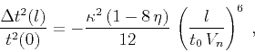 |
(50) |
while the error of the shifted-hyperbola approximation
(30) is
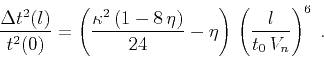 |
(51) |
Comparing
equations (50) and (51), we
conclude that if the medium is elliptically anisotropic  ,
the shifted hyperbola can be twice as accurate as the anisotropic equation
(assuming the optimal choice of parameters). The accuracy of the latter,
however, increases when the anellipticity coefficient grows and
becomes higher than that of the shifted hyperbola if satisfies
the approximate inequality
,
the shifted hyperbola can be twice as accurate as the anisotropic equation
(assuming the optimal choice of parameters). The accuracy of the latter,
however, increases when the anellipticity coefficient grows and
becomes higher than that of the shifted hyperbola if satisfies
the approximate inequality
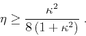 |
(52) |
For instance, if
 , inequality (52) yields
 , a quite small value.
|
|
|
|
| Nonhyperbolic reflection moveout of -waves:
An overview and comparison of reasons | |
|
Next: CURVILINEAR REFLECTOR
Up: VERTICAL HETEROGENEITY
Previous: Vertically heterogeneous isotropic model
2014-01-27
![$\displaystyle {1 \over t_z}\,\int_{0}^{t_z}\,V_z^{2}(t)\,
\left[1 + 2\,\delta(t)\right]\,dt\;,$](img104.png)
![$\displaystyle {1 \over t_z}\,\int_{0}^{t_z}\,V_z^{2k}(t)\,
\left[1 + 2\,\delta(t)\right]^{2k}\,\left[1 + 8\,\eta(t)\right]\,dt \qquad
(k = 2,3, \ldots)\;.$](img105.png)