|
|
|
|
Time-shift imaging condition in seismic migration |

|
|---|
|
hyper
Figure 3. An image is formed when the Kirchoff stacking curve (dashed line) touches the true reflection response. Left: the case of under-migration; right: over-migration. |
|
|

|
|---|
|
off
Figure 4. Common-image gathers for space-shift imaging (left column) and time-shift imaging (right column). |
|
|

|
|---|
|
ssk
Figure 5. Common-image gathers after slant-stack for space-shift imaging (left column) and for time-shift imaging (right column). The vertical line indicates the migration velocity. |
|
|
We can use the Kirchhoff formulation to analyze the moveout behavior of the time-shift imaging condition in the simplest case of a flat reflector in a constant-velocity medium (Figures 3-5).
The synthetic data are imaged using shot-record
wavefield extrapolation migration.
Figure 4 shows offset
common-image gathers for three different migration
slownesses ![]() , one of which is equal to the
modeling slowness
, one of which is equal to the
modeling slowness ![]() .
The left column corresponds to the space-shift imaging condition
and the right column corresponds to the time-shift imaging condition.
.
The left column corresponds to the space-shift imaging condition
and the right column corresponds to the time-shift imaging condition.
For the space-shift CIGs imaged with correct slowness, left column in Figure 4, the energy is focused at zero offset, but it spreads in a region of offsets when the slowness is wrong. Slant-stacking produces the images in left column of Figure 5.
For the time-shift CIGs imaged with correct slowness, right column in Figure 4, the energy is distributed along a line with a slope equal to the local velocity at the reflector position, but it spreads around this region when the slowness is wrong. Slant-stacking produces the images in the right column of Figure 5.
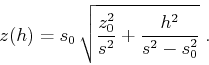
Let ![]() and
and ![]() represent
the true slowness and reflector depth, and
represent
the true slowness and reflector depth, and ![]() and
and ![]() stand for the
corresponding quantities used in migration. An image is formed when
the Kirchoff stacking curve
stand for the
corresponding quantities used in migration. An image is formed when
the Kirchoff stacking curve
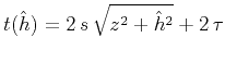 touches the true reflection response
 (Figure 3).
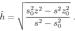
Solving for
(Figure 3).
Solving for ![]() from the envelope condition
from the envelope condition
![]() yields two solutions:
yields two solutions:
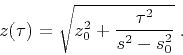
By contrast, the moveout shape ![]() appearing in wave-equation
migration with the lateral-shift imaging condition is (Bartana et al., 2005)
appearing in wave-equation
migration with the lateral-shift imaging condition is (Bartana et al., 2005)
|
|
|
|
Time-shift imaging condition in seismic migration |