Interferometric imaging condition for wave-equation migration

Statistical stability

The interferometric imaging condition described in the preceding section is used to reduce imaging artifacts by attenuating the incoherent energy corresponding to velocity errors, as illustrated in Figures 6(b) and 6(d). The random model used for this example corresponds to the weak fluctuation regime, as explained in Appendix A (characteristic wavelength of similar scale with the random fluctuations in the medium and fluctuations with small magnitude).

By statistical instability we mean that images obtained for different realizations of random models with the identical statistics are different. Figures 7(a)-7(c) illustrate data modeled for different realizations of the random model in Figure 3(b). The general kinematics of the data are the same, but subtle differences exist between the various datasets due to the random model variations. Migration using a conventional imaging condition leads to the images in Figures 7(d)-7(f) which also show variations from one realization to another. In contrast, Figures 7(g)-7(i) show images obtained by the interferometric imaging condition in equations 5-8, which are more similar to one-another since many of the artifacts have been attenuated.

pdv-r0,pdv-r1,pdv-r2,winpcic-r0,winpcic-r1,winpcic-r2,winpiic-r0,winpiic-r1,winpiic-r2
Figure 7. Illustration of statistical stability for the interferometric imaging condition in presence of random model variations. Data modeled using velocity with random variations of magnitude $\sigma=30\%$, for different realizations of the noise model $n$. Images obtained by conventional imaging (d)-(f) and images obtained by interferometric imaging (g)-(i).

In typical seismic imaging problems, we cannot ensure that random velocity fluctuations are small (e.g. $\sigma\le 5\%$). It is desirable that imaging remains statistically stable even in cases when velocity varies with larger magnitude. We investigate the statistical properties of the imaging functional in equations 5-8 using numerical experiments similar to the one used earlier. We describe the random noise present in the velocity models using the following parameters explained in Appendix A: seismic spatial wavelength $\lambda=76.2$ m, wavelet central frequency $\omega=20$ Hz, random fluctuations parameters: $r_a=0.0762$, $r_c=0.0762$, $\alpha=2$, and random noise magnitude $\sigma$ between $15\%$ and $45\%$. This numerical experiment simulates a situation that mixes the theoretical regimes explained in Appendix B: random model fluctuations of comparable scale with the seismic wavelength lead to destruction of the wavefronts, as suggested by the ``weak fluctuations'' regime; large magnitude of the random noise leads to diffusion of the wavefronts, as suggested by the ``diffusion approximation'' regime. This combination of parameters could be regarded as a worst-case-scenario from a theoretical standpoint.

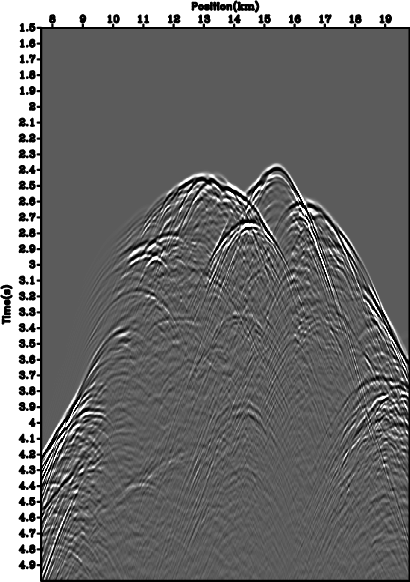
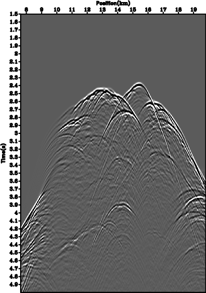
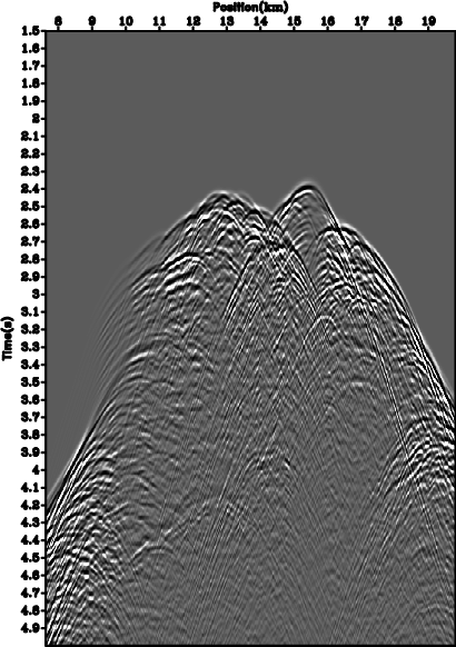
Figures 8(a)-8(c) show data simulated in models similar to the one depicted in Figure 3(b), but where the random noise component is described by $\sigma=15,30,45\%$, respectively. As expected, the wavefronts recorded at the surface are increasingly distorted to the point where some of the later arrival are not even visible in the data.

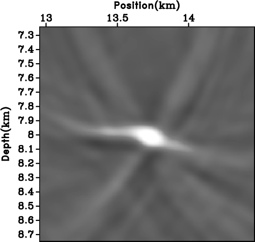
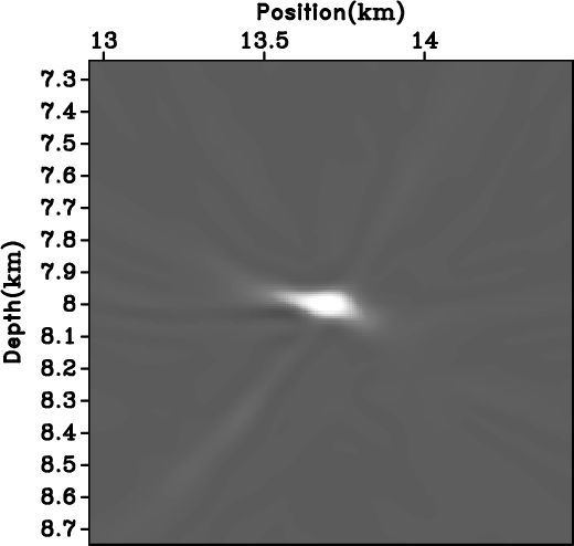
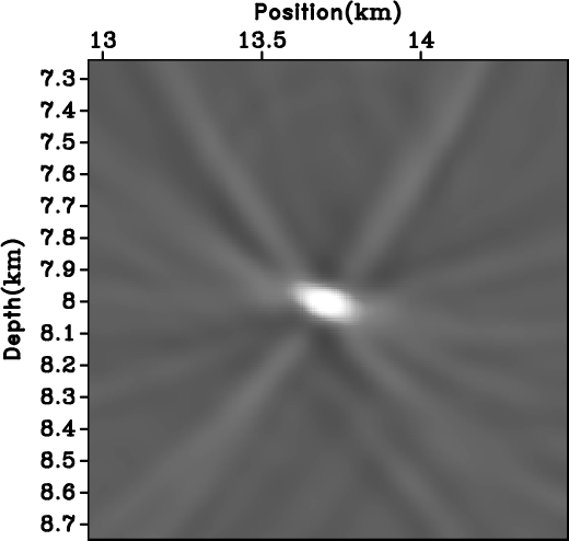
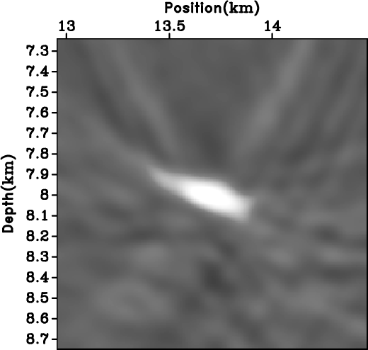
Migration using a conventional imaging condition leads to the images in Figures 8(d)-8(f). As expected, the images show stronger artifacts due to the larger defocusing caused by the unknown random fluctuations in the model. However, migration using the interferometric imaging condition leads to the images in Figures 8(g)-8(i). Artifacts are significantly reduced and the images are much better focused.

pdv-m0,pdv-m1,pdv-m2,winpcic-m0,winpcic-m1,winpcic-m2,winpiic-m0,winpiic-m1,winpiic-m2
Figure 8. Illustration of interferometric imaging condition robustness in presence of random model variations. Data modeled using velocity with random variations of magnitudes $\sigma=15\%$ (a), $\sigma=30\%$ (b), and $\sigma=45\%$ (c). Images obtained by conventional imaging (d)-(f) and images obtained by interferometric imaging (g)-(i).

Interferometric imaging condition for wave-equation migration