Elastic wave-mode separation for VTI media

Separation method

Separation of scalar and vector potentials can be achieved by Helmholtz decomposition, which is applicable to any vector field $\mathbf W(x,y,z)$ . By definition, the vector wavefield $\mathbf W$ can be decomposed into a curl-free scalar potential $\Theta$ and a divergence-free vector potential $\boldsymbol \Psi$ according to the relation (Aki and Richards, 2002):

$$\mathbf W= \nabla \Theta + \nabla \times {\boldsymbol \Psi} .$$ (1)

Equation 1 is not used directly in practice, but the scalar and vector components are obtained indirectly by the application of the $\nabla \cdot {}$ and $\nabla \times {}$ operators to the extrapolated elastic wavefield:

$$P = \nabla \cdot {\mathbf W} ,$$ (2)

$$\mathbf S = \nabla \times {\mathbf W} .$$ (3)

For isotropic elastic fields far from the source, quantities $P$ and $\mathbf S$ describe compressional and shear wave modes, respectively (Aki and Richards, 2002).

Equations 2 and 3 allow one to understand why $\nabla \cdot {}$ and $\nabla \times {}$ pass compressional and transverse wave modes, respectively. In the discretized space domain, one can write:

$$P= \nabla \cdot {\mathbf W} = D_x[W_x]+D_y[W_y]+D_z[W_z] ,$$ (4)

where $D_x$ , $D_y$ , and $D_z$ represent spatial derivatives in the $x$ , $y$ , and $z$ directions, respectively. Applying derivatives in the space domain is equivalent to applying finite difference filtering to the functions. Here, $D\left [\cdot\right]$ represents spatial filtering of the wavefield with finite difference operators. In the Fourier domain, one can represent the operators $D_x$ , $D_y$ , and $D_z$ by $i k_x$ , $i k_y$ , and $i k_z$ , respectively; therefore, one can write an equivalent expression to equation 4 as:

$$\widetilde{\mathbf P}=i \mathbf k\cdot \widetilde{\mathbf W}= i k_x \widetilde W_x+i k_y \widetilde W_y+i k_z \widetilde W_z ,$$ (5)

where $\mathbf k=\{k_x,k_y,k_z\}$ represents the wave vector, and $\widetilde{\mathbf W}(k_x,k_y,k_z)$ is the 3D Fourier transform of the wavefield $\mathbf W(x,y,z)$ . We see that in this domain, the operator $i \mathbf k$ essentially projects the wavefield $\widetilde{\mathbf W}$ onto the wave vector $\mathbf k$ , which represents the polarization direction for P waves. Similarly, the operator $\nabla \times {}$ projects the wavefield onto the direction orthogonal to the wave vector $\mathbf k$ , which represents the polarization direction for S waves (Dellinger and Etgen, 1990). For illustration, Figure 1(a) shows the polarization vectors of the P mode of a 2D isotropic model as a function of normalized $k_x$ and $k_z$ ranging from $-1$ to $1$ cycles. The polarization vectors are radial because the P waves in an isotropic medium are polarized in the same directions as the wave vectors.

Iso-polarvector,Ani-polarvector
Figure 1. The qP and qS polarization vectors as a function of normalized wavenumbers $k_x$ and $k_z$ ranging from $-1$ to $+1$ cycles, for (a) an isotropic model with $V_P=3$  km/s and $V_S=1.5$  km/s, and (b) an anisotropic (VTI) model with $V_{P0}=3$  km/s, $V_{S0}=1.5$  km/s, $\epsilon=0.25$ and $\delta=-0.29$ . The red arrows are the qP wave polarization vectors, and the blue arrows are the qS wave polarization vectors.

Dellinger and Etgen (1990) suggest the idea that wave mode separation can be extended to anisotropic media by projecting the wavefields onto the directions in which the P and S modes are polarized. This requires that one should modify the wave separation equation 5 by projecting the wavefields onto the true polarization directions U to obtain quasi-P (qP) waves:

$$\widetilde {{\it q}P}=i \mathbf U(\mathbf k) \cdot \widetilde{\... ...W} =i U_x \widetilde W_x+i U_y \widetilde W_y+i U_z \widetilde W_z .$$ (6)

In anisotropic media, $\mathbf U(k_x,k_y,k_z)$ is different from $\mathbf k$ , as illustrated in Figure 1(b), which shows the polarization vectors of qP wave mode for a 2D VTI anisotropic model with normalized $k_x$ and $k_z$ ranging from $-1$ to $1$ cycles. Polarization vectors are not radial because qP waves in an anisotropic medium are not polarized in the same directions as wave vectors, except in the symmetry planes ($k_z=0$ ) and along the symmetry axis ($k_x=0$ ).

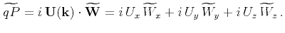
Dellinger and Etgen (1990) demonstrate wave mode separation in the wavenumber domain using projection of the polarization vectors, as indicated in equation 6. However, for heterogeneous media, this equation is defective because the polarization vectors are spatially varying. One can write an equivalent expression to equation 6 in the space domain for each grid point as:

$${\it q}P=\nabla_a\cdot \mathbf W= L_x[W_x] + L_y[W_y] + L_z[W_z] ,$$ (7)

where $L_x$ , $L_y$ , and $L_z$ represent the inverse Fourier transforms of $i U_x$ , $i U_y$ , and $i U_z$ , respectively. $L\left[\cdot\right]$ represents spatial filtering of the wavefield with anisotropic separators. $L_x$ , $L_y$ , and $L_z$ define the pseudo derivative operators in the $x$ , $y$ , and $z$ directions for an anisotropic medium, respectively, and they change from location to location according to the material parameters.

We obtain the polarization vectors $\mathbf U(\mathbf k)$ by solving the Christoffel equation (Aki and Richards, 2002; Tsvankin, 2005):

$$\left [{\bf G} - \rho V^2 {\bf I} \right]\mathbf U= 0 ,$$ (8)

where G is the Christoffel matrix $G_{ij}=c_{ijkl}n_jn_l$ , in which $c_{ijkl}$ is the stiffness tensor, $n_j$ and $n_l$ are the normalized wave vector components in the $j$ and $l$ directions, $i,j,k,l=1,2,3$ . The parameter $V$ corresponds to the eigenvalues of the matrix G. The eigenvalues $V$ represent the phase velocities of different wave modes and are functions of the wave vector $\mathbf k$ (corresponding to $n_j$ and $n_l$ in the matrix G). For plane waves propagating in any symmetry planes of a VTI medium, one can set $k_y$ to 0 and get

$$\left [ \mtrx{ c_{11} k_x^2 +c_{55} k_z^2 -\rho V^2 &0& \left (c_... ...c_{33} k_z^2 -\rho V^2 } \right] \left [\mtrx{ U_x\ U_y\ U_z} \right] =0 .$$ (9)

The middle row of this matrix characterizes the SH wave polarized in the $y$ direction, and qP and qSV modes are uncoupled from the SH mode and are polarized in the vertical plane. The top and bottom rows of this equation allow one to compute the polarization vector $\mathbf U=\{U_x,U_z\}$ (the eigenvectors of the matrix ) of P or SV wave mode given the stiffness tensor at every location of the medium.

One can extend the procedure described here to heterogeneous media by computing two different operator for each mode at every grid point. In the symmetry planes of VTI media, the operators are 2D and depend on the local values of the stiffness coefficients. For each point, I pre-compute the polarization vectors as a function of the local medium parameters, and transform them to the space domain to obtain the wave mode separators. I assume that the medium parameters vary smoothly (locally homogeneous), but even for complex media, the localized operators work in the same way as the long finite difference operators. If one represents the stiffness coefficients using Thomsen parameters (Thomsen, 1986), then the pseudo derivative operators $L_x$ and $L_z$ depend on $\epsilon$ , $\delta$ , $V_{P0}$ and $V_{S0}$ , which can be spatially varying parameters. One can compute and store the operators for all grid points in the medium, and then use these operators to separate P and S modes from reconstructed elastic wavefields at different time steps. Thus, wavefield separation in VTI media can be achieved simply by non-stationary filtering with operators $L_x$ and $L_z$ .

Elastic wave-mode separation for VTI media