Wide-azimuth angle gathers for wave-equation migration

Imaging conditions

Conventional seismic imaging is based on the concept of single scattering. Under this assumption, waves propagate from seismic sources, interact with discontinuities and return to the surface as reflected seismic waves. We commonly speak about a ``source'' wavefield, originating at the seismic source and propagating in the medium prior to any interaction with discontinuities, and a ``receiver'' wavefield, originating at discontinuities and propagating in the medium to the receivers (Berkhout, 1982; Clærbout, 1985). The two wavefields kinematically coincide at discontinuities.

We can formulate imaging as a process involving two steps: the wavefield reconstruction and the imaging condition. The key elements in this imaging procedure are the source and receiver wavefields, ${W_s}$ and ${W_r}$ which are $4$ -dimensional objects as a function of space ${\bf x}=\{x,y,z\}$ and time $t$ , or as a function of space and frequency $\omega$ . For imaging, we need to analyze if the wavefields match kinematically in time and then extract the reflectivity information using an imaging condition operating along the space and time axes.

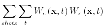
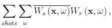
A conventional cross-correlation imaging condition (cIC) based on the reconstructed wavefields can be formulated in the time or frequency domain as the zero lag of the cross-correlation between the source and receiver wavefields (Clærbout, 1985):

$$R\left ({\bf x}\right) = \sum\limits_{shots} \sum\limits_{t} {W_s}\left ({\bf x}, t \right) {W_r}\left ({\bf x}, t \right)$$ (1)

$$= \sum\limits_{shots} \sum\limits_{\omega } \overline{ {W_s}\left ({\bf x}, \omega \right)} {W_r}\left ({\bf x}, \omega \right),$$ (2)

where $R$ represents the migrated image and the over-line represents complex conjugation. This operation exploits the fact that portions of the source and receiver wavefields match kinematically at subsurface positions where discontinuities occur. Alternative imaging conditions use deconvolution of the source and receiver wavefields, but we do not elaborate further on this subject since the differences between cross-correlation and deconvolution are not central for this paper.

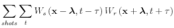
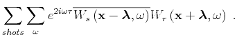
An extended imaging condition preserves in the output image certain acquisition (e.g. source or receiver coordinates) or illumination (e.g. reflection angle) parameters (Weglein and Stolt, 1999; Clayton and Stolt, 1981; Clærbout, 1985; Stolt and Weglein, 1985). In shot-record migration, the source and receiver wavefields are reconstructed on the same computational grid at all locations in space and all times or frequencies, therefore there is no a-priori wavefield separation that can be transferred to the output image. In this situation, the separation can be constructed by correlation of the wavefields from symmetric locations relative to the image point, measured either in space (Rickett and Sava, 2002; Sava and Fomel, 2005) or in time (Sava and Fomel, 2006). This separation essentially represents local cross-correlation lags between the source and receiver wavefields. Thus, an extended cross-correlation imaging condition (eIC) defines the image as a function of space and cross-correlation lags in space and time. This imaging condition can also be formulated in the time and frequency domains (Sava and Vasconcelos, 2011):

$$R\left ({\bf x}, {\boldsymbol{\lambda}} , \tau \right) = \sum\limits_{shots} \sum\limits_{t} {W_s}\left ({\bf x}- {\boldsy... ...} , t-\tau \right) {W_r}\left ({\bf x}+ {\boldsymbol{\lambda}} , t+\tau \right)$$ (3)

$$= \sum\limits_{shots} \sum\limits_{\omega } e^{2 i \omega \tau } \o... ...omega \right)} {W_r}\left ({\bf x}+ {\boldsymbol{\lambda}} , \omega \right)\;.$$ (4)

Equations 1-2 represent a special case of equations 3-4 for ${\boldsymbol{\lambda}} =0$ and $\tau =0$ . Assuming that all errors accumulated in the incorrectly-reconstructed wavefields are due to the velocity model, the extended images could be used for velocity model building by exploiting semblance properties emphasized by the space-lags (Sava and Biondi, 2004a; Shen et al., 2003; Biondi and Sava, 1999; Sava and Biondi, 2004b) and focusing properties emphasized by the time-lag (MacKay and Abma, 1993; Faye and Jeannot, 1986; Nemeth, 1995,1996; MacKay and Abma, 1992). Furthermore, these extensions can be converted to reflection angles (Sava and Fomel, 2006; Weglein and Stolt, 1999; Sava and Fomel, 2003), thus enabling analysis of amplitude variation with angle for images constructed in complex areas using wavefield-based imaging.

Typically, angle decomposition with extended images uses common image gathers, i.e. representations of (a subset of) the extensions as a function of a space axis, typically the depth axis. As pointed out by Sava and Vasconcelos (2011), this approach suffers from major drawbacks. Common-image-gathers are appropriate for nearly horizontal structures and they are computationally wasteful since they require un-necessary calculations, e.g. inside massive salt bodies. In contrast, the common-image-point-gathers advocated by Sava and Vasconcelos (2011) are constructed at selected points in the image, thus eliminating unnecessary calculations, and they can accomodate arbitrary orientations of the reflectors.

In this paper, we use extended common-image-point-gathers to extract angle-dependent reflectivity at individual points in the image. The method described in the following section is appropriate for 3D wide-azimuth wave-equation imaging. The problem we are solving is to decompose extended CIPs as a function of azimuth $\phi$ and reflection $\theta$ angles at selected points in the image. In general, the input for such decomposition are gathers in the $\{ {\boldsymbol{\lambda}} ,\tau \}$ domain, and the output are gathers in the $\{\phi,\theta,\tau \}$ domain:

$$R\left ( {\boldsymbol{\lambda}} ,\tau \right)\Longrightarrow R\left (\phi,\theta,\tau \right)\;.$$ (5)

Here we address a special case of this decomposition which is appropriate for imaging with correct velocity. In this case, all the energy in the output CIPs concentrates at $\tau =0$ , so we can focus our attention on a particular case of the decomposition which does not preserve the time-lag variable in the output: $R\left ( {\boldsymbol{\lambda}} ,\tau \right)\Longrightarrow R\left (\phi,\theta \right)$ . We omit the dependence of the extended images on space (${\bf x}$ ) to highlight the fact that the decomposition can be performed independently at various points in the image. The topic of angle decomposition when the gathers are constructed with incorrect velocity remains outside the scope of this paper. However, we note that the angle decomposition in such situation is not necessary, since semblance optimization can be implemented based on the image extensions directly (Shen and Symes, 2008; Symes, 2009).

In the remainder of the paper, we show that all the necessary information for this decomposition is available after wave-equation migration, regardless of its implementation, e.g by depth or time extrapolation. A pre-requisite for this decomposition is the moveout function characterizing individual shots, as discussed in the following section. We then show how the moveout information can be used for angle decomposition and illustrate the method with simple and complex synthetic examples.

Wide-azimuth angle gathers for wave-equation migration