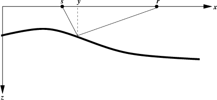
next up previous [pdf]

Next: Computational part Up: Homework 3 Previous: Homework 3

Theoretical part

  1. In class, we derived the following acoustic wave equation for pressure $P(\mathbf{x},t)$:
    \begin{displaymath}
{\frac{1}{V^2(\mathbf{x})}}\,{\frac{\partial^2 P}{\partial t...
...nabla\left(\frac{1}{\rho(\mathbf{x})}\right) \cdot \nabla P\;.
\end{displaymath} (1)

    1. Using the connection between the pressure and displacement, derive the acoustic wave equation for the displacement vector $\mathbf{u}(\mathbf{x},t)$:
      \begin{displaymath}
\rho(\mathbf{x})\,\frac{\partial^2 \mathbf{u}}{\partial t^2} =
\end{displaymath} (2)

    2. Consider a geometrical wave representation in the vicinity of a wavefront
      \begin{displaymath}
{\mathbf{u}(\mathbf{x},t)} = \mathbf{a}(\mathbf{x})\,f\left(t-T(\mathbf{x})\right)
\end{displaymath} (3)

      and derive partial differential equations for the traveltime function $T(\mathbf{x})$ and the vector amplitude $\mathbf{a}(\mathbf{x})$.

    3. Assuming that the geometrical wave propagates in the direction of the traveltime gradient
      \begin{displaymath}
{\mathbf{a}(\mathbf{x})} = A(\mathbf{x})\,V(\mathbf{x})\,\nabla T
\end{displaymath} (4)

      show that the amplitude continuation along a ray is given by equation
      \begin{displaymath}
\left\vert\mathbf{a}_1\right\vert = \left\vert\mathbf{a}_...
...eft(\frac{\rho_0\,V_0\,J_0}{\rho_1\,V_1\,J_1}\right)^{1/2}\;,
\end{displaymath} (5)

      where $J_0$ and $J_1$ are the corresponding geometrical spreading factors.

  2. Consider a medium with a constant gradient of slowness squared
    \begin{displaymath}
S^2(\mathbf{x}) = S_0^2 + 2\,\mathbf{g} \cdot (\mathbf{x}-\mathbf{x}_0)\;.
\end{displaymath} (6)

    1. In the 2-D case, the ray-family coordinate system can be specified by $\mathbf{r}=\{\sigma,\theta\}$, where $\sigma$ goes along the ray, and $\theta$ is the initial ray angle. A family of rays starts from the source point $\mathbf{x}_0$, with each ray traveling in the direction $\mathbf{p_0} =
\{S_0\,\cos{\theta},S_0\,\sin{\theta}\}$. Show that the coordinate transformation matrix $\mathbf{P}=\partial \mathbf{p}/\partial
\mathbf{r}$ changes along the ray as
      \begin{displaymath}
\mathbf{P}(\sigma) = \left[\begin{array}{cc}
g_1 & -S_0...
...in{\theta} \\
g_2 & S_0\,\cos{\theta} \end{array}\right]\;,
\end{displaymath} (7)

      where $g_1$ and $g_2$ are the components of $\mathbf{g}$ and find the corresponding transformation of matrices $\mathbf{X}=\partial \mathbf{x}/\partial \mathbf{r}$ and $\mathbf{K}=\mathbf{P}\,\mathbf{X}^{-1}$.
      $\displaystyle \mathbf{X}(\sigma)$ $\textstyle =$   (8)
      $\displaystyle \mathbf{K}(\sigma)$ $\textstyle =$   (9)

  3. Consider the source point $s$ and the receiver point $r$ at the surface $z=0$ above a 2-D constant-velocity medium and a curved reflector defined by the equation $z = z(x)$ with a twice differentiable function $z(x)$ (Figure 1).

    curve
    curve
    Figure 1.
    Geometry of reflection in a constant-velocity medium with a curved reflector.
    [pdf] [png] [xfig]

    Note that the two-point ray trajectory can be parametrized by the reflection point $y$ with the following expression for the reflection traveltime (using the Pythagoras theorem):

    \begin{displaymath}
T(s,r) = {\frac{\sqrt{(s-y)^2+z^2(y)}+\sqrt{(r-y)^2+z^2(y)}}{V}}\;.
\end{displaymath} (10)

    1. Apply Fermat's principle to specify $F(y)$ in the equation
      \begin{displaymath}
F(y) = 0
\end{displaymath} (11)

      required for finding the reflection point $y$.

    2. Newton's method (successive linearization) solves nonlinear equations like (11) iteratively by starting with some $y_0$ and repeating the iteration
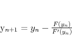
      \begin{displaymath}
y_{n+1} = y_n - \frac{F(y_n)}{F'(y_n)}
\end{displaymath} (12)

      for $n=0,1,2,\ldots$

      Specify $F'(y)$ for the problem of finding the reflection point.

    3. Consider the special case of a dipping-plane reflector
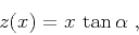
      \begin{displaymath}
z(x) = x\,\tan{\alpha}\;,
\end{displaymath} (13)

      where $\alpha$ is the dip angle. Show that, in this case, equation (11) reduces to a linear equation for $y$. Find $y$ and substitute it into (10) to define the reflection traveltime analytically.

    4. (EXTRA CREDIT) Find the reflection traveltime for a circle reflector
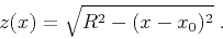
      \begin{displaymath}
z(x) = \sqrt{R^2 - (x-x_0)^2}\;.
\end{displaymath} (14)


next up previous [pdf]

Next: Computational part Up: Homework 3 Previous: Homework 3

2019-10-10