Next: Conclusions Up: Song & Fomel: FFD Previous: Theory

Numerical Examples

Our first example is a comparison of four methods: the 4th-order finite differences, pseudo-spectral method, velocity interpolation, and the FFD method in a velocity model with smooth variation, formulated as

$\displaystyle v(x,z)\,=\,550+1.5\times10^{-4}(x-800)^2+10^{-4}(z-500)^2;$

$\displaystyle 0\le x\le2560,\;0\le z\le2560.$

The velocity is between 550 m/s and 1439 m/s. A Ricker-wavelet source with maximum frequency 70 Hz is located at the center of the model. For all the numerical simulations based on this model, we use the same grid size: $\Delta x\,=\,5$ m and $\Delta t\,=\,2$ ms.

Figure 3(a) shows an obvious numerical dispersion from the snapshot of the acoustic wavefield computed by the 4th-order finite difference method. Figure 3(b) shows a slight dispersion from the snapshot computed by pseudo-spectral method (Reshef et al., 1988b). Figure 3(c) shows the corresponding snapshot of the velocity-interpolation method (Etgen and Brandsberg-Dahl, 2009; Crawley et al., 2010), calculated using two reference velocities. It is practically free of dispersion thanks to spectral compensation. Figure 3(d) shows a snapshot of the proposed FFD method. It is almost exactly the same as Figure 3(c); however, only one reference velocity is used instead of two. As comparison between Figure 3(d) and Figure 3(c) implies, the FFD method has practically the same accuracy as the velocity interpolation method while having only one reference velocity and therefore replacing the cost of one additional FFT with the cost of a low-order finite-difference operator.


wavfd,wavsp,wavpspi,wavffd Figure 3. Acoustic wavefield snapshot by: (a) 4th-order Finite Difference method; (b) pseudo-spectral method; (c) velocity interpolation method with 2 reference velocities; (d) FFD method with RMS velocity.

Our next example is a snapshot of the acoustic wavefield calculated by FFD in the BP model (Billette and Brandsberg-Dahl, 2004). We use a Ricker-wavelet at a point source. The maximum frequency is 50 Hz. The horizontal grid size $\Delta x$ is 37.5 m, the vertical grid size $\Delta z$ is 12.5 m and the time step is 1 ms. Figure 4 shows a part of the model with a salt body. Figure 5 shows a wavefield snapshot confirming that the FFD method can work in a complex-velocity medium as well.


vel Figure 4. Portion of BP 2004 synthetic velocity model.


wavsnap Figure 5. Wavefield snapshot in the BP Model shown in Figure 4.

Next we apply our FFD algorithm to RTM with a simple exponential decaying boundary condition (Cerjan et al., 1985). The dominant frequency is 27 Hz. The space grid is 25 m and the time step is 1.5 ms. Figure 6 shows the output image. The inner and outer flanks of the salt body are clearly imaged.


img Figure 6. RTM image of BP salt model.

The cost advantage of FFD is even more appealing in anisotropic (TTI) media, which require multiple velocity parameters and increase the cost of velocity interpolation. Figure 7 shows the impulse response of a 4th-order FFD operator in a TTI model with the tilt of $45\,^{\circ}$ and a smooth velocity variation ( : 800-1225.41 m/s, : 700-883.6 m/s). The space grid size is 5 m and the time step is 1 ms. Note no coupling of qP-waves and qSV-waves (Zhang et al., 2009) in the figure, thanks to the Fourier construction of the operator.

For this paper, we implemented a 2nd-order 5-point FD scheme for 2D isotropic case. One can observe little dispersion in isotropic examples. For TTI media, we use a 13-point scheme which minimizes the error in the symmetry plane and in the direction normal to the symmetry plane. One can still see some dispersion in the corresponding snapshot; which indicates that a higher order FD scheme might be required to further supress the dispersion.


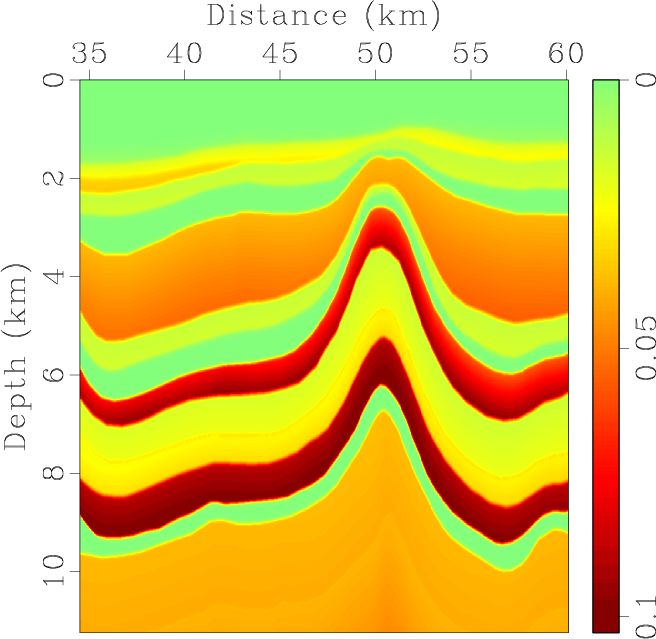
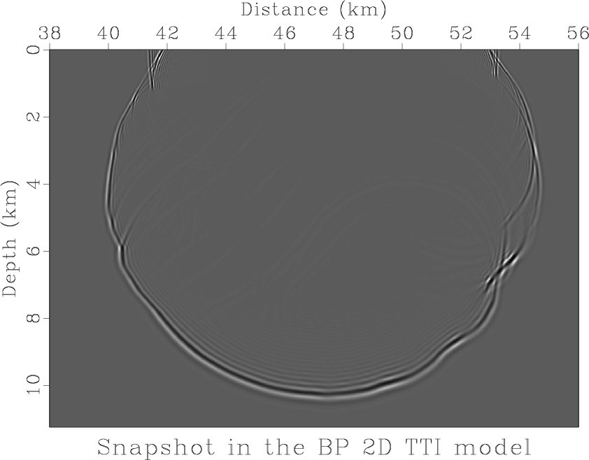
TTI-snapshot Figure 7. Wavefield snapshot in a TTI medium with tilt of 45 degrees. $v_x(x,z)=800+10^{-4}(x-1000)^2+10^{-4}(z-1200)^2$ ; $v_z(x,z)=700+10^{-4}(z-1200)^2$ ; $\eta =0.3$ ; $\theta=45\,^{\circ}$ .

Our last example is qP-wave simulation in the BP 2D TTI model. Figure 8(a)-8(d) shows parameters for part of the model. The maximum frequency is 50 Hz. The space grid size is 12.5 m and the time step is 1 ms. The snapshot of the acoustic wavefield in Figure 9 demonstrates the stability of our approach in a complicated anisotropic model. Some small dispersion is present in the TTI examples, pointing to a possible need to extend the FD part of the FFD scheme from second order to higher orders.