Antialiasing of Kirchhoff operators by reciprocal parameterization

Proposed technique

We can use the reciprocity of the time parameterization and the space parameterization of integral operators, discovered by Hale, to arrive at the following antialiasing technique.

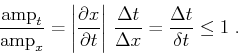
For simplicity, let us consider the two-dimensional case first. The linearity of a two-dimensional integral operator allows us to decompose this operator into two parts. The first part corresponds to the steep part of the travel-time function, which satisfies the time-sampling criterion (4). The second term corresponds to the flat part of the traveltime, which satisfies the space-sampling criterion (1). The first part is not aliased with respect to the time sampling interval, while the second one is not aliased with respect to the space sampling. We can apply interpolation in time to construct the flat part. Reciprocally, interpolation in space is applied to construct the steep part of the operator in the fashion of Hale's time-shifting method. The amplitude difference between the two integrals is simply the Jacobian term

$${\mbox{amp}_t \over \mbox{amp}_x}= \left\vert{\partial x \ov... ...{\Delta t \over \Delta x}= {\Delta t \over \delta t} \leq 1\;.$$ (5)

According to the proposed modification, Hale's antialiasing principle is reformulated, as follows:

In the steep part of an integral operator, never allow successive time shifts applied to the input trace to differ by more than one time sampling interval. In the flat part of the operator, never allow successive space shifts to differ by more than one space sampling interval.

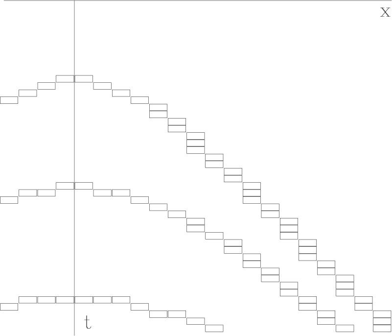
Figure 4, borrowed from Claerbout (1995), illustrates the basic idea of the proposed technique. It clearly shows the difference between the flat and steep parts of migration hyperbolas. To observe the reciprocity, rotate the figure by 90 degrees.

amotra
Figure 4. Figure borrowed from Claerbout (1995) to illustrate the reciprocity antialiasing. The flat parts of the hyperbolas require interpolation in time. The steep parts of the hyperbolas require interpolation in space.

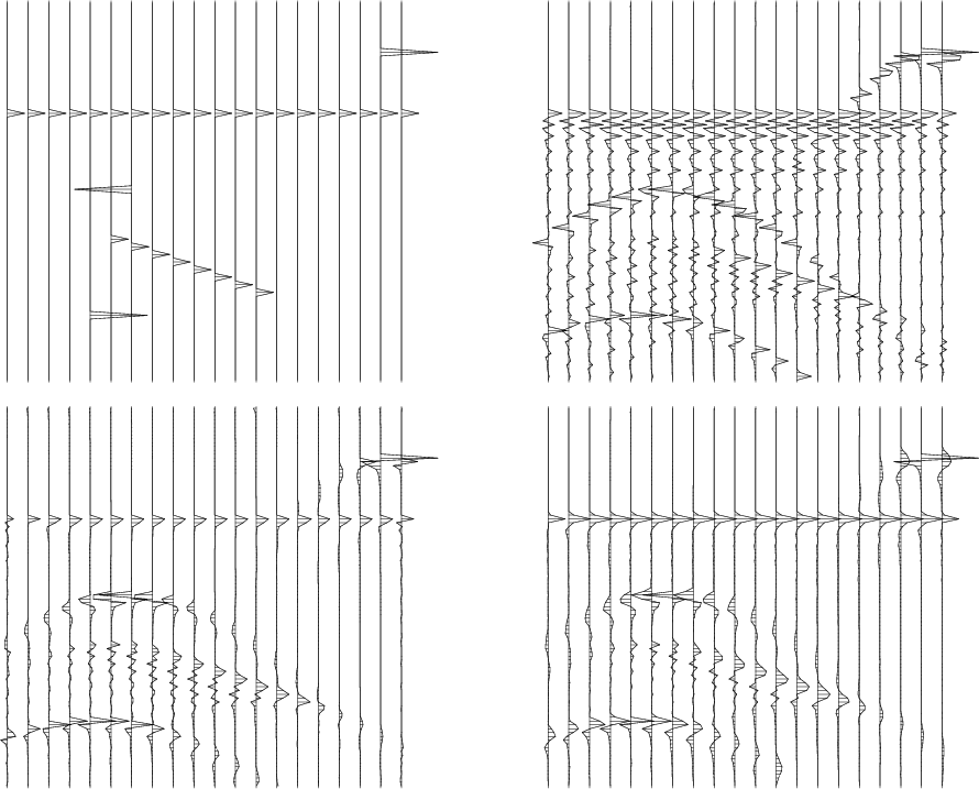
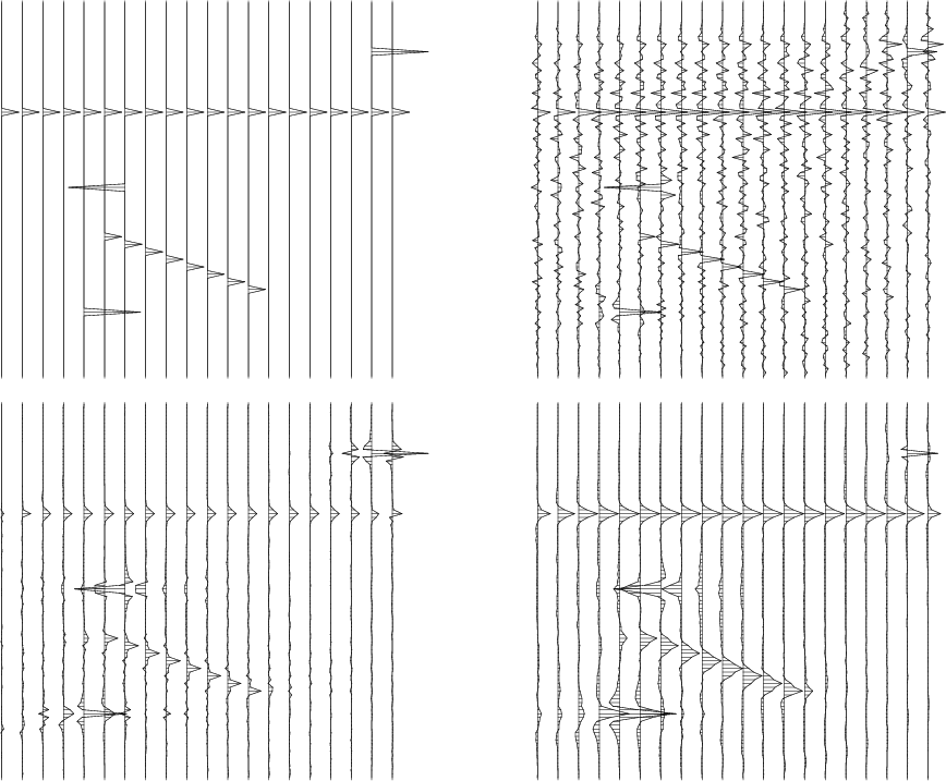
To compare the proposed antialiasing method with the temporal filtering method, I test the antialiased migration program on simple 2-D synthetic tests. Figure 5 shows a simple model and the modeling results from modeling without antialiasing, with temporal filtering, and with the proposed reciprocity method. The modeling results were migrated with the corresponding migration operators to obtain the image of the model in Figure 6. Both the temporal filtering and the proposed method succeed in removing the major aliasing artifacts. However, the reciprocity method demonstrates a higher resolution and a better preservation of the frequency content.

amomod
Figure 5. Top left is a synthetic model. Top right is modeling without antialiasing. Bottom left is modeling with reciprocity antialiasing (the proposed method). Bottom right is modeling with antialiasing by temporal filtering.

amomig
Figure 6. Top left plot is the synthetic model. The other plots are migrations of the corresponding data shown in the previous figure . Top right is a migration without antialiasing. Bottom left is a migration with reciprocity antialiasing (the proposed method). Bottom right is a migration with triangle filter antialiasing.

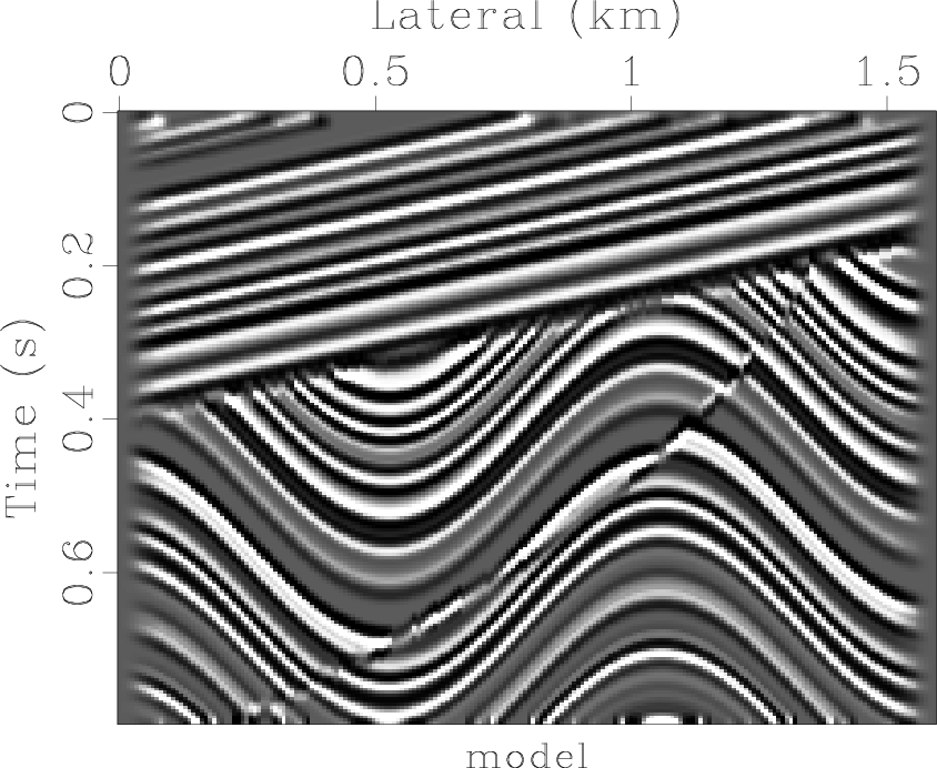
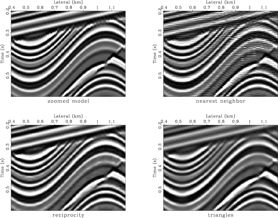
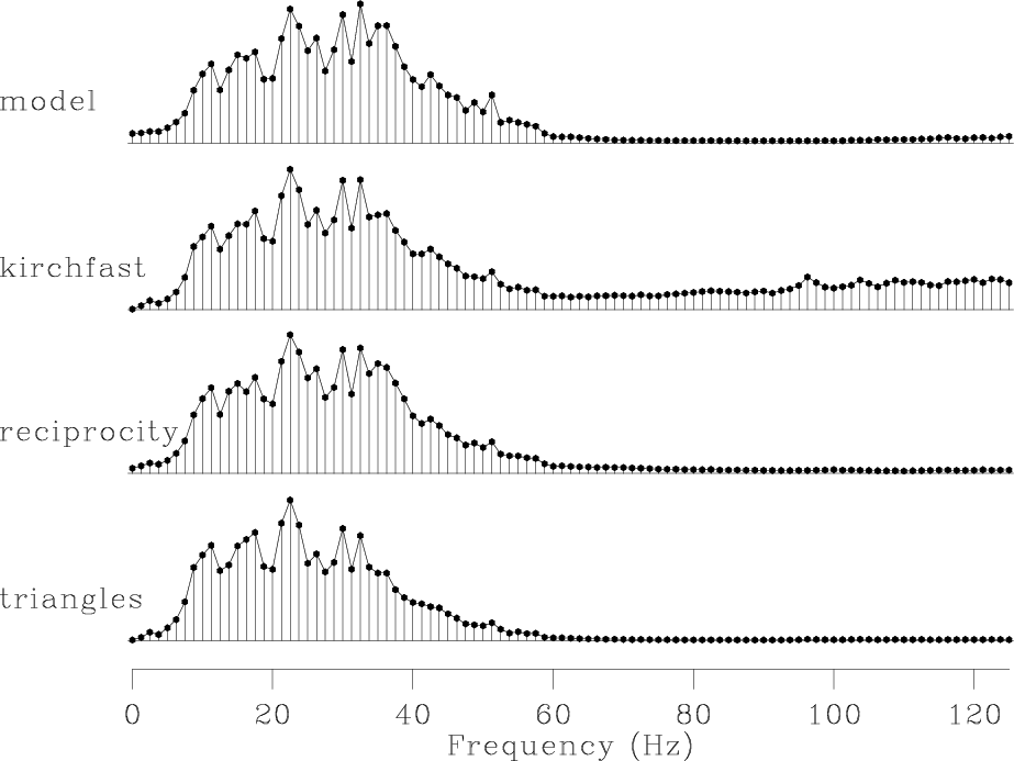
These properties are examined more closely in the next synthetic example. Figure 7 shows a more sophisticated synthetic model that contains a fault, an unconformity and layered structures (Claerbout, 1995). For better displaying, I extract the central part of the model and compare it with the migration results of different methods in Figure 8. Comparing the plots shows that the reciprocity method successfully removes the aliasing artifacts (round-off errors) of the aliased (nearest neighbor interpolation) migration. At the same time, it is less harmful to the high-frequency components of the data than triangle filtering. This conclusion finds an additional support in Figure 9 that displays the average spectrum of the image traces for different methods. Both of the antialiasing methods remove the high-frequency artifacts of the nearest neighbor modeling and migration. The reciprocity method performs it in a gentler way, preserving the high-frequency components of the model.

amosmo
Figure 7. Synthetic model used to test the antialiased migration program.

amosmi
Figure 8. Top left plot is a zoomed portion of the synthetic model. The other plots are migrated images. Top right is a migration without antialiasing. Bottom left is a migration with reciprocity antialiasing (the proposed method). Bottom right is a migration with triangle filter antialiasing.

amospe
Figure 9. Top is the spectrum of the model. The other plots are the spectra of the migrated images. The second plot corresponds to the modeling/migration without account for antialiasing. The third plot is modeling/migration with the reciprocity antialiasing. The bottom plot is modeling/migration with triangle antialiasing.

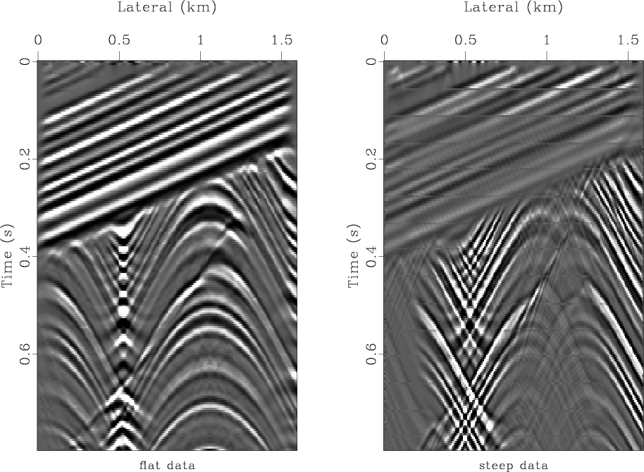
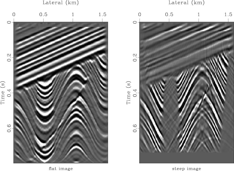
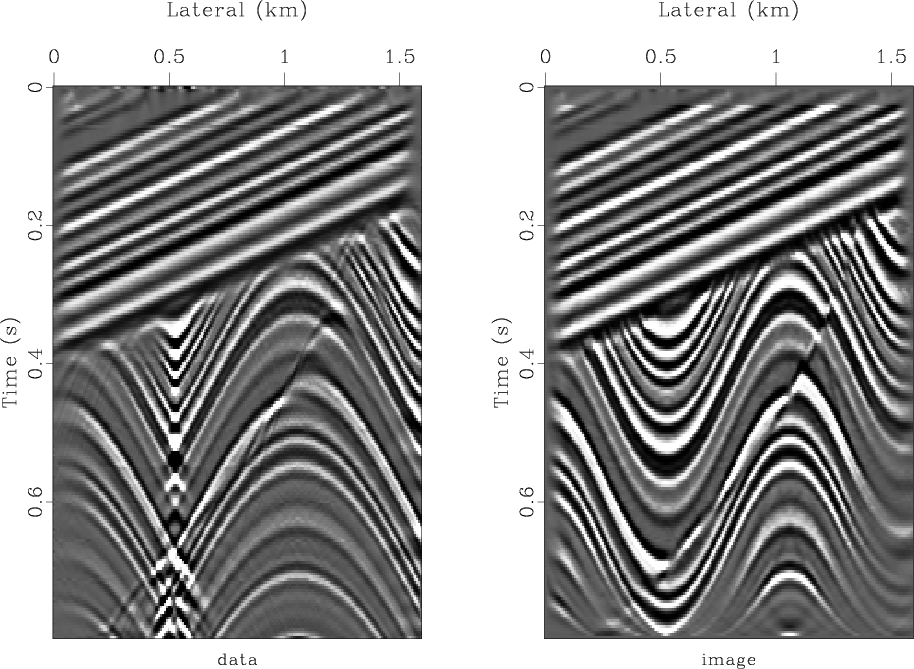
The algorithm sequence of the antialiased migration is illustrated in Figures 10 and 11. The two plots in Figure 10 show the steep-dip and flat-dip modeling respectively. The superposition of these two terms is the resultant antialiased data shown in the left plot of Figure 12. The right plot of Figure 12 shows the migrated image obtained by adding the flat-dip (left of Figure 11) and steep-dip (right of Figure 11) migrations.

amormo
Figure 10. Antialiased modeling. Left corresponds to the flat-dip term. Right corresponds to the steep-dip term.

amormi
Figure 11. Antialiased migration. Left corresponds to the flat-dip term. Right corresponds to the steep-dip term.

amormm
Figure 12. Antialiased modeling and migration. Left is the superposition of the flat-dip and steep-dip modeling. Right is superposition of the flat-dip and steep-dip migration.

Antialiasing of Kirchhoff operators by reciprocal parameterization