Iterative least-square inversion for amplitude balancing

AMPLITUDE BALANCING

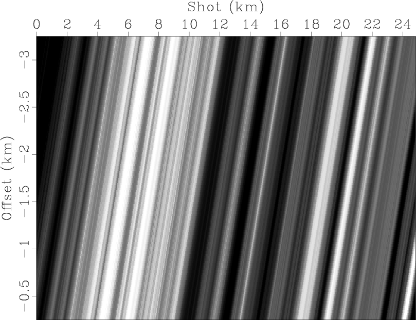
We use the coefficients calculated for the source, offset, and receiver directions to remove the stripes from the plot in Figure 1. Figure 8 shows the 2-D synthetic amplitude map modeled using the source and offset coefficient curves only. The similarity between the stripes in the amplitude plots in Figures 1 and 8 is quite strong.

sostripes
Figure 8. Synthetic 2-D amplitude map modeled using the source and offset coefficients.

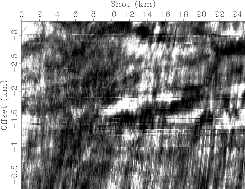
We divide the original 2-D amplitude function by the source and offset correction coefficients to obtain the amplitude map in Figure 9. In this plot most of the source- and offset-related anomalous amplitude stripes seem to have disappeared, revealing the grey background (the earth impulse response and noise) and other stripes dipping to the left.

sobalcd
Figure 9. 2-D amplitude map corrected for variations in the source and offset directions using the coefficient curves in Figures 4 and 5.

Comparing Figure 9 and the modeled stripes in Figure 2, we can associate the now more apparent dipping stripes with the receiver- and midpoint-consistent stripes. In Figure 9, the fine stripes with a steep dip particularly visible at the bottom part of the plot can be regarded as midpoint-consistent, whereas the less steep stripes are receiver-related.

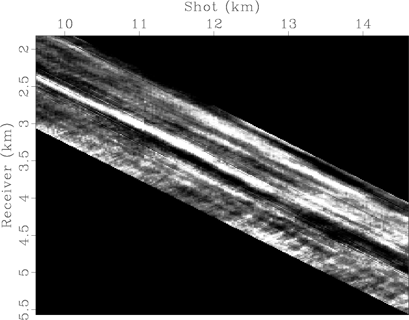
Figure 10 represents a portion of the amplitude map in Figure 9 in the source and receiver coordinate system. The plot shows a bright spot smeared along the offset direction (the descending diagonal). Two very broad darker stripes orthogonal to the receiver axis are visible around the receiver positions at 9.5 km and 12 km. In this coordinate system we can identify these two broad stripes as receiver-consistent. This observation is confirmed by Figure 7, in which the receiver correction coefficient curve shows two local minima at the corresponding receiver location. The same stripes are also noticeable in the center of the plot in Figure 9, though less obvious. They are also clearly visible in Figure 11, which is a synthetic amplitude map modeled from the receiver coefficients only.

srsobalcd
Figure 10. Portion of the amplitude map in Figure 9 displayed in the source and receiver space.

rvstripes
Figure 11. Synthetic 2-D amplitude map modeled using the receiver coefficients.

Figure 12 shows the amplitude map corrected for variations in the source, offset, and receiver directions. It is the result of the division of the plot in Figure 9 by the estimated receiver coefficients in Figure 7. Figure 13 represents the portion of the corrected amplitude map in Figure 12 in the source and receiver coordinate system. After the correction has been applied, the broad horizontal stripes around the receiver positions at 9.5 km and 12 km have disappeared.

balanced
Figure 12. 2-D amplitude map corrected for variations in the source, offset, and receiver directions using the coefficient curves in Figures 4, 5, and 7.

srbalanced
Figure 13. Portion of the corrected amplitude map in Figure 12 displayed in the source and receiver space.

Although midpoint-consistent factors are not used to correct the data amplitudes, we invert for the factors simultaneously to separate the different components more fully. The resulting amplitude map, corrected for anomalous variations in the source, offset, and receiver directions, shows the contribution of the earth and midpoint components to the amplitude of the recorded traces. Some variations may still be present, but not dominant.

Iterative least-square inversion for amplitude balancing