Multi-dimensional Fourier transforms in the helical coordinate system

Wavenumber in helical coordinates

With the understanding that the 1-D FFT of a multi-dimensional signal in helical coordinates is equivalent to the 2-D FFT, a natural question to ask is: how does the helical wavenumber, $k_h$, relate to spatial wavenumbers, $k_x$ and $k_y$?

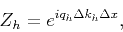
The helical delay operator, $Z_h$, is related to $k_h$ through the equation,

$$Z_h = e^{i k_h \Delta x}.$$ (8)

In the discrete frequency domain this becomes

$$Z_h = e^{i q_h \Delta k_h \Delta x},$$ (9)

where $q_h$ is the integer frequency index that lies in the range, $0 \leq q_h < N_x N_y$. The uncertainty relationship, $\Delta k_h \Delta x = \frac{2 \pi}{N_x N_y}$, allows this to be simplified still further, leaving

$$Z_h = e^{2 \pi i \; \frac{q_h}{N_x N_y}}.$$ (10)

If we find a form of $q_h$ in terms of Fourier indices, $q_x$ and $q_y$, that can be plugged into equation (10) in order to satisfy equations (4) and (5), this will provide the link between $k_h$ and spatial wavenumbers, $k_x$ and $k_y$.

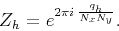
The idea that $x$-axis wavenumbers will have a higher frequency than $y$-axis wavenumbers, leads us to try a $q_h$ of the form,

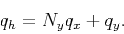$$q_h = N_y q_x + q_y.$$ (11)

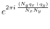
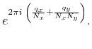
Substituting this into equation (10) leads to

$$Z_h = e^{2 \pi i \; \frac{(N_y q_x + q_y)}{N_x N_y}}$$ (12)

$$= e^{2 \pi i \; \left( \frac{q_x}{N_x} + \frac{q_y}{N_x N_y} \right)}.$$ (13)

Since $q_y$ is bounded by $N_y$, for large $N_x$ the second term in braces $\frac{q_y}{N_x N_y} \approx 0$, and this reduces to

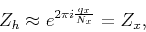$$Z_h \approx e^{2 \pi i \frac{q_x}{N_x}} = Z_x,$$ (14)

which satisfies equation (4).

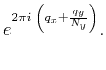
Substituting equation (11) into equation (10), and raising it to the power of $N_x$ leads to:

$$Z_h^{N_x} = e^{2 \pi i \frac{(N_y q_x + q_y)}{N_y}}$$ (15)

$$= e^{2 \pi i \; \left( q_x + \frac{q_y}{N_y} \right)}.$$ (16)

Since $q_x$ is an integer, $e^{2 \pi i q_x} = 1$, and this reduces to

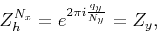$$Z_h^{N_x} = e^{2 \pi i \frac{q_y}{N_y}} = Z_y,$$ (17)

which satisfies equation (5).

Equation (11), therefore, provides the link we are looking for between $q_x$, $q_y$, and $q_h$. It is interesting to note that not only is there a one-to-one mapping between 1-D and 2-D Fourier components, but equation (11) describes helical boundaries in Fourier space: however, rather than wrapping around the $x$-axis as it does in physical space, the helix wraps around the $k_y$-axis in Fourier space (Figure 2). This provides the link that is missing in Figure 1, but shown in Figure 3.

transp Figure 2. Fourier dual of helical boundary conditions is also helical boundary conditions with axis of helix transposed.

ill2 Figure 3. Relationship between 1-D and 2-D convolution, FFT's and the helix, illustrating the Fourier dual of helical boundary conditions.

As with helical coordinates in physical space, equation (11) can easily be inverted to yield

$$k_x = \Delta k_x q_x = \frac{2 \pi}{N_x \Delta x} \left[ \frac{q_h}{N_y}\right], \hspace{0.25in} {\rm and}$$ (18)

$$k_y = \Delta k_y q_y = \frac{2 \pi}{N_y \Delta y} \left( q_h - N_y \left[ \frac{q_h}{N_y}\right] \right)$$ (19)

where $[x]$ denotes the integer part of $x$.

Multi-dimensional Fourier transforms in the helical coordinate system