Post-Stack Time Migration

Next: Velocity Transform Up: EXAMPLES Previous: 3. Common-offset migration

Post-Stack Time Migration

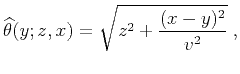
An interesting example of a stacking operator is the hyperbola summation used for time migration in the post-stack domain. In this case, the summation path is defined as

$\displaystyle \widehat{\theta}(y;z,x) = \sqrt{z^2+{{(x-y)^2}\over {v^2}}}\;,$

(59)

where

denotes the vertical traveltime,

and

are the horizontal coordinates on the migrated and unmigrated sections respectively, and

stands for the effectively constant root-mean-square velocity (Claerbout, 1995). The summation path for the reverse transformation (demigration) is found from solving equation (59) for

. It has the well-known elliptic form

$\displaystyle \theta(x;t,y) = \sqrt{t^2-{{(x-y)^2}\over {v^2}}}\;.$

(60)

The Jacobian of transforming

$\displaystyle \left\vert\partial \widehat{\theta} \over \partial z\right\vert = {z \over t}\;.$

(61)

If the migration weighting function is defined by conventional downward continuation (Schneider, 1978), it takes the following form, which is equivalent to equation (40):

$\displaystyle \widehat{w}(y;z,x) = {1\over{\left(2 \pi\right)^{m/2}}} {{\co... ...= {1\over{\left(2 \pi\right)^{m/2}}} {\cos{\alpha} \over {v^m t^{m/2}}}\;.$

(62)

The simple trigonometry of the reflected ray suggests that the cosine factor in formula (62) is equal to the simple ratio between the vertical traveltime

and the zero-offset reflected traveltime

$\displaystyle \cos{\alpha} = {z \over t}\;.$

(63)

The equivalence of the Jacobian (61) and the cosine factor (63) has important interpretations in the theory of Stolt frequency-domain migration (Levin, 1986; Chun and Jacewitz, 1981; Stolt, 1978). According to equation (22), the weighting function of the adjoint operator is the ratio of (62) and (61):

$\displaystyle \widetilde{w}(x;t,y) = {1\over{\left(2 \pi\right)^{m/2}}} {1 \over {v^m t^{m/2}}}\;.$

(64)

We can see that the cosine factor

disappears from the adjoint weighting. This is completely analogous to the known effect of ``dropping the Jacobian'' in Stolt migration (Harlan, 1983; Levin, 1994). The product of the weighting functions for the time migration and its asymptotic inverse is defined according to formula (10) as

$\displaystyle w \widehat{w}={1\over{\left(2 \pi\right)^m}} {\sqrt{\left\ve... ...al \widehat{\theta} \over \partial z\right\vert^m}} = {1 \over {(v^2 t)^m}}\;.$

(65)

Thus, the asymptotic inverse of the conventional time migration has the weighting function determined from equations (10) and (62) as

$\displaystyle w(x;t,y) = {1\over{\left(2 \pi\right)^{m/2}}} {{t/z} \over {v^m t^{m/2}}}\;.$

(66)

The weighting functions of the asymptotic pseudo-unitary operators are obtained from formulas (28) and (29). They have the form

$\displaystyle w^{(+)}(x;t,y)$	$\displaystyle =$	$\displaystyle {1\over{\left(2 \pi\right)^{m/2}}} {\sqrt{t/z} \over {v^m t^{m/2}}}\;.$	(67)
$\displaystyle w^{(-)}(y;z,x)$	$\displaystyle =$	$\displaystyle {1\over{\left(2 \pi\right)^{m/2}}} {\sqrt{z/t} \over {v^m t^{m/2}}}\;.$	(68)

The square roots of the cosine factor appearing in formulas (67) and (68) correspond to the analogous terms in the pseudo-unitary Stolt migration proposed by Harlan and Sword (1986).

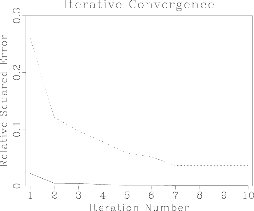
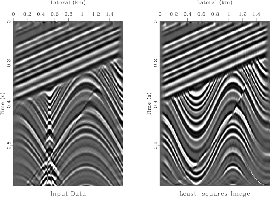
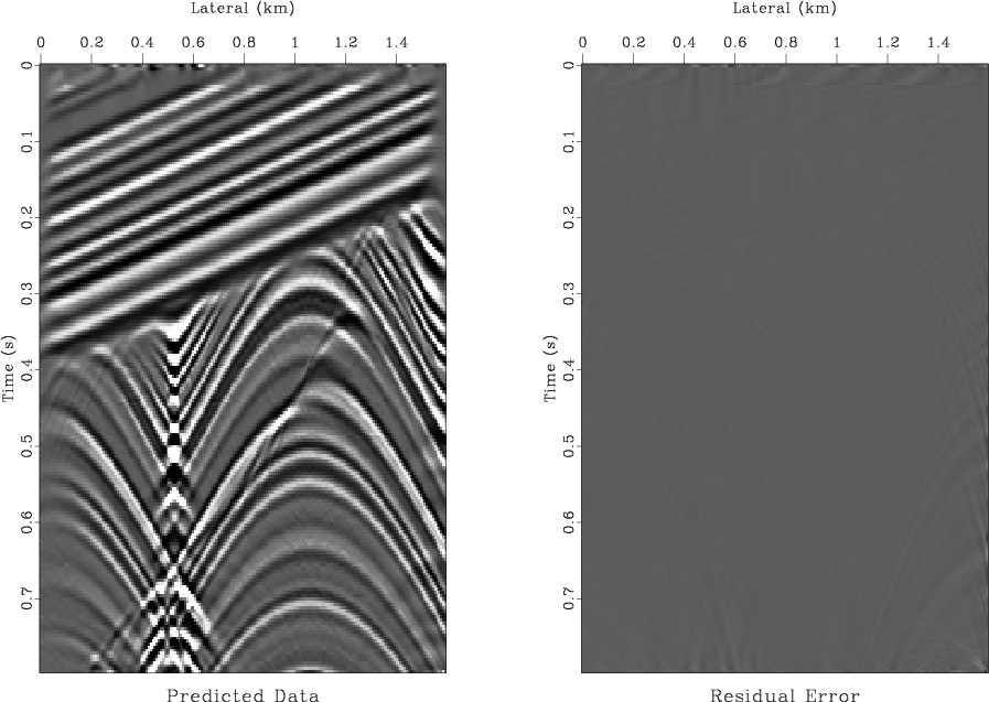
Figure 1 shows the output of a simple numerical test. The synthetic zero-offset section used in this test is shown in the left plot of Figure 2. The data are taken from Claerbout (1995) and correspond to a synthetic reflectivity model, which contains several dipping layers, a fault, and an unconformity. The input zero-offset section is inverted using an iterative conjugate-gradient method and two different weighting schemes: the uniform weighting and the asymptotic pseudo-unitary weighting (67-68). I compare the iterative convergence by measuring the least-squares norm of the data residual error at different iterations. Figure 1 shows that the pseudo-unitary weighting provides a significantly faster convergence. The result of inversion after 10 conjugate-gradient iterations is shown in Figures 2 and 3. The right plot in Figure 2 shows the output of the least-squares migration. Figure 3 shows the corresponding modeled data and the residual error. The latter is very close to zero. Although this example has only a pedagogical value, it clearly demonstrates possible advantages of using asymptotic pseudo-unitary operators in least-squares migration.

migiter Figure 1. Comparison of convergence of the iterative least-squares migration. The dashed line corresponds to the unweighted (uniformly weighted) operator. The solid line corresponds to the asymptotic pseudo-unitary operator. The latter provides a noticeably faster convergence.


migcvv Figure 2. Input zero-offset section (left) and the corresponding least-squares image (right) after 10 iterations of iterative inversion.


migrst Figure 3. The modeled zero-offset (left) and the residual error (right) plotted at the same scale.

Next: Velocity Transform Up: EXAMPLES Previous: 3. Common-offset migration

2013-03-03