 |
 |
 |
 | Asymptotic pseudounitary stacking operators |  |
![[pdf]](icons/pdf.png) |
Next: 1. Common-shot migration
Up: EXAMPLES
Previous: Datuming
Least-squares migration, envisioned by Lailly (1984) and
Tarantola (1984), has recently
become a practical method and gained a lot of attention in the
geophysical literature (Nemeth et al., 1999; Fomel et al., 2002; Chavent and Plessix, 1999; Duquet and Marfurt, 1999). Using the
theory of asymptotic pseudo-unitary operators allows us to reconcile
this approach with the method of asymptotic true-amplitude
migration (Bleistein et al., 2001).
As recognized by Tygel et al. (1994), true-amplitude migration
(Schleicher et al., 1993; Goldin, 1992) is the asymptotic inversion of seismic modeling
represented by the Kirchhoff high-frequency approximation. The
Kirchhoff approximation for a reflected wave (Bleistein, 1984; Haddon and Buchen, 1981)
belongs to the class of stacking-type operators (1)
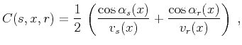
with the summation path
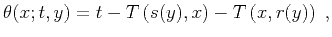 |
(41) |
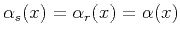
the weighting function
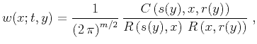 |
(42) |
and the additional time filter
 . Here
  denotes a point at the reflector surface,
 is the source location, and
  is the receiver location at the
observation surface. The parameter
is the receiver location at the
observation surface. The parameter  corresponds to the
configuration of observation. That is,
corresponds to the
configuration of observation. That is,
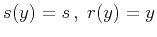 for the
common-shot configuration,
for the
common-shot configuration,
 for the zero-offset
configuration, and
for the zero-offset
configuration, and
 for the
common-offset configuration (where
for the
common-offset configuration (where  is the half-offset). The
functions
is the half-offset). The
functions  and
and  have the same meaning as in the datuming example,
representing the one-way traveltime and the one-way geometric
spreading, respectively. The function
have the same meaning as in the datuming example,
representing the one-way traveltime and the one-way geometric
spreading, respectively. The function  is known as the obliquity factor. Its definition is
 |
(43) |
where the angles
 and
and
 are formed by the
incident and reflected waves with the normal to the reflector at the
point
, and
are formed by the
incident and reflected waves with the normal to the reflector at the
point
, and  and
and  are the corresponding velocities
in the vicinity of this point. In this paper, I leave the case of
converted (e.g., P-SV) waves outside the scope of consideration and
assume that
equals
(e.g., in P-P reflection). In this
case, it is important to notice that at the stationary point of the
Kirchhoff integral,
are the corresponding velocities
in the vicinity of this point. In this paper, I leave the case of
converted (e.g., P-SV) waves outside the scope of consideration and
assume that
equals
(e.g., in P-P reflection). In this
case, it is important to notice that at the stationary point of the
Kirchhoff integral,
 (the law of
reflection), and therefore
(the law of
reflection), and therefore
 |
(44) |
The stationary point of the Kirchhoff integral is the point where the
stacking curve (41) is tangent to the actual reflection
traveltime curve. When our goal is asymptotic inversion, it is
appropriate to use equation (44) in place of
(43) to construct the inverse operator. The weighted
function (42) can include other factors affecting the
leading-order (WKBJ) ray amplitude, such as the source signature,
caustics counter (the KMAH-index), and transmission coefficient
for the interfaces (Chapman and Drummond, 1982; Cerveny, 2001). In the following analysis,
I neglect these factors for simplicity.
The model  implied by the Kirchhoff modeling integral is the
wavefield with the wavelet shape of the incident wave and the
amplitude proportional to the reflector coefficient along the
reflector surface. The goal of true-amplitude migration is to recover
from the observed seismic data. In order to obtain the image of
the reflectors, the reconstructed model is evaluated at the time
implied by the Kirchhoff modeling integral is the
wavefield with the wavelet shape of the incident wave and the
amplitude proportional to the reflector coefficient along the
reflector surface. The goal of true-amplitude migration is to recover
from the observed seismic data. In order to obtain the image of
the reflectors, the reconstructed model is evaluated at the time  equal to zero. The Kirchhoff modeling integral requires explicit
definition of the reflector surface. However, its inverse doesn't
require explicit specification of the reflector location. For each
point of the subsurface, one can find the normal to the hypothetical
reflector by bisecting the angle between the
equal to zero. The Kirchhoff modeling integral requires explicit
definition of the reflector surface. However, its inverse doesn't
require explicit specification of the reflector location. For each
point of the subsurface, one can find the normal to the hypothetical
reflector by bisecting the angle between the  and
and  rays. Born scattering approximation provides a different physical
model for the reflected waves. According to this approximation, the
recorded waves are viewed as scattered on smooth local inhomogeneities
rather than reflected from sharp reflector surfaces. The inversion of
Born modeling (Miller et al., 1987; Bleistein, 1987) closely
corresponds with the result of Kirchhoff integral inversion. For an
unknown reflector and the correct macro-velocity model, the asymptotic
inversion reconstructs the signal located at the reflector surface
with the amplitude proportional to the reflector coefficient.
rays. Born scattering approximation provides a different physical
model for the reflected waves. According to this approximation, the
recorded waves are viewed as scattered on smooth local inhomogeneities
rather than reflected from sharp reflector surfaces. The inversion of
Born modeling (Miller et al., 1987; Bleistein, 1987) closely
corresponds with the result of Kirchhoff integral inversion. For an
unknown reflector and the correct macro-velocity model, the asymptotic
inversion reconstructs the signal located at the reflector surface
with the amplitude proportional to the reflector coefficient.
As follows from the form of the summation path (41), the
integral migration operator must have the summation path
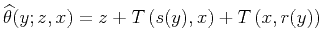 |
(45) |
to reconstruct the geometry of the reflector at the migrated section.
According to equation (8), the asymptotic
reconstruction of the wavelet requires, in addition, the derivative
filter
 . The
asymptotic reconstruction of the amplitude defines the true-amplitude
weighting function in accordance with equation (10), as
follows:
. The
asymptotic reconstruction of the amplitude defines the true-amplitude
weighting function in accordance with equation (10), as
follows:
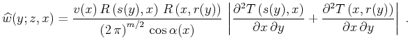 |
(46) |
The weighting function of the asymptotic pseudo-unitary migration is
found analogously to equation (34) as
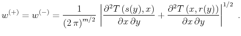 |
(47) |
Unlike true-amplitude migration, this type of migration operator
does not change the dimensionality of the input. Several specific cases exist
for different configurations of the input data.
Subsections
|
|
|
|
| Asymptotic pseudounitary stacking operators | |
|
Next: 1. Common-shot migration
Up: EXAMPLES
Previous: Datuming
2013-03-03