|
|
|
|
First-break traveltime tomography with the double-square-root eikonal equation |
The numerical examples in this section serve several different purposes. The first example will test the accuracy of modified FMM DSR eikonal equation solver (DSR FMM) and show the drawbacks of the alternative explicit discretization. The second example will demonstrate effect of considering non-causal branches of DSR eikonal equation in forward modeling. The third example will compare the sensitivity kernels of DSR tomography and standard tomography in a simple model. The last example will present a tomographic inversion and demonstrate advantages of DSR method over the traditional method.
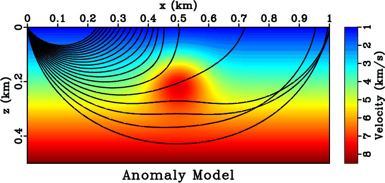
Figure 5 shows a 2-D velocity model with a constant-velocity-gradient background plus a Gaussian
anomaly in the middle. We use ![]() to denote the grid spacing in
to denote the grid spacing in ![]() and
and ![]() in
in ![]() . The
traveltimes on the surface
. The
traveltimes on the surface ![]() km of a shot at
km of a shot at ![]() km are computed by DSR FMM at a gradually refined
km are computed by DSR FMM at a gradually refined
![]() or
or ![]() while fixing the other one. For reference, we also calculate first-breaks
by a second-order FMM (Popovici and Sethian, 2002; Rickett and Fomel, 1999) for the same shot at a very fine grid spacing of
while fixing the other one. For reference, we also calculate first-breaks
by a second-order FMM (Popovici and Sethian, 2002; Rickett and Fomel, 1999) for the same shot at a very fine grid spacing of
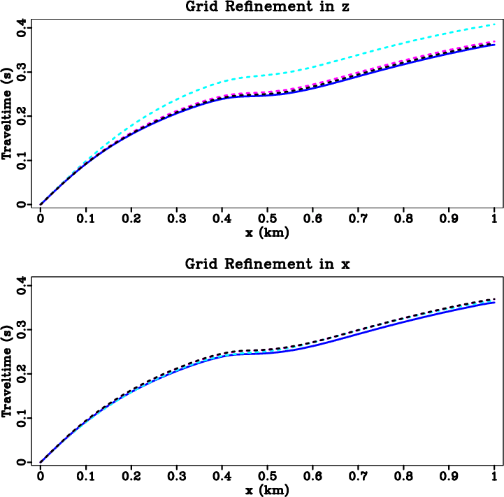
![]() m. In Figure 6, a
grid refinement in both
m. In Figure 6, a
grid refinement in both ![]() and
and ![]() helps reducing errors of the implicit discretization, although
improvements in the
helps reducing errors of the implicit discretization, although
improvements in the ![]() refinement case are less significant because the majority of the ray-paths are
non-horizontal. The results are consistent with the analysis in Appendix A, which shows
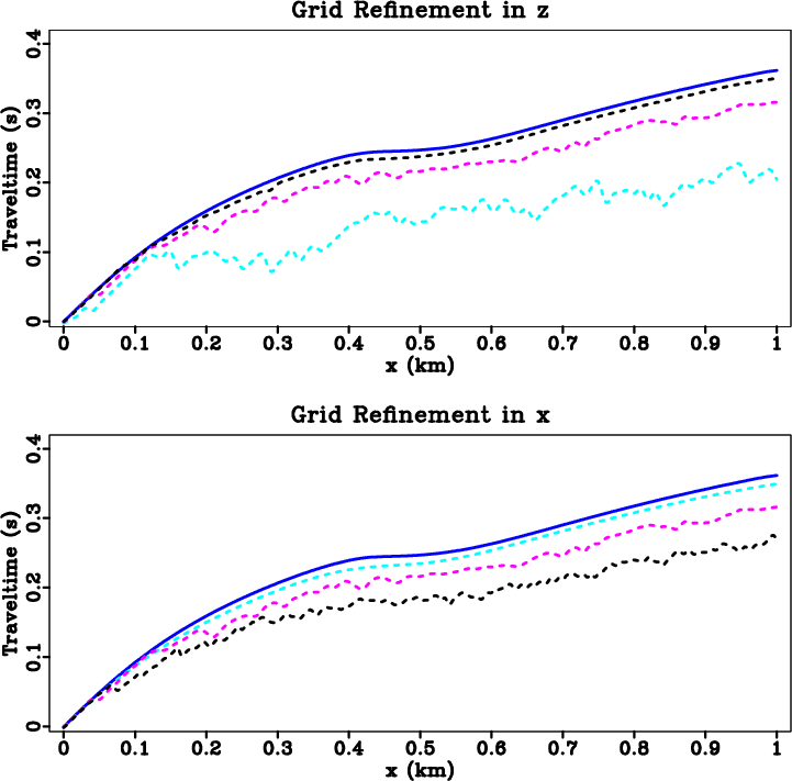
that the implicit discretization is unconditionally convergent. On the other hand, as shown in
Figure 7, the explicit discretization is only conditionally convergent when
refinement case are less significant because the majority of the ray-paths are
non-horizontal. The results are consistent with the analysis in Appendix A, which shows
that the implicit discretization is unconditionally convergent. On the other hand, as shown in
Figure 7, the explicit discretization is only conditionally convergent when
![]() under grid refinement in order to resolve the flatter parts of the ray-paths. This
explains why its accuracy deteriorates when refining
under grid refinement in order to resolve the flatter parts of the ray-paths. This
explains why its accuracy deteriorates when refining ![]() and fixing
and fixing ![]() . A more detailed error analysis
remains open for future research.
. A more detailed error analysis
remains open for future research.
|
|---|
|
modl
Figure 5. The synthetic model used for DSR FMM accuracy test. The overlaid curves are rays traced from a shot at |
|
|
|
|---|
|
imp
Figure 6. Grid refinement experiment (implicit discretization). In both figures, the solid blue curve is the reference values and the dashed curves are computed by DSR FMM. Top: fixed |
|
|
|
|---|
|
exp
Figure 7. Grid refinement experiment (explicit discretization). The experiment set-ups are the same as in Figure 6. |
|
|
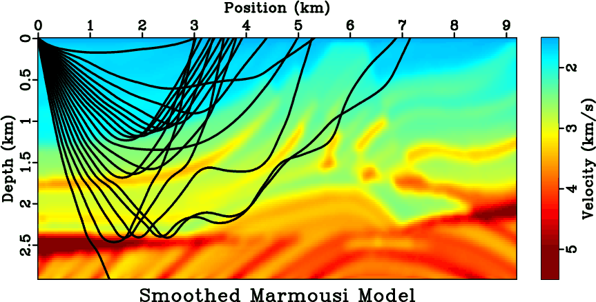
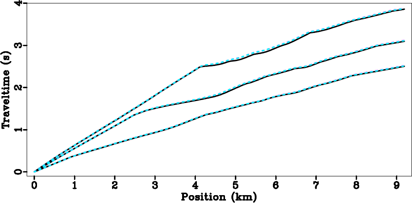
Next, we use a smoothed Marmousi model (Figure 8) and run two DSR FMMs, one with the search
process for non-causal DSR branches turned-on and the other turned-off. In Figure 9, again we
compute reference values by a second-order FMM. The three groups of curves are
traveltimes of shots at ![]() km,
km, ![]() km and
km and ![]() km, respectively. The maximum absolute
differences between the two DSR FMMs, for all three shots, are approximately
km, respectively. The maximum absolute
differences between the two DSR FMMs, for all three shots, are approximately ![]() ms at the largest offset. This
shows that, if the near-surface model is moderately complex, then the first-breaks are of causal
types described by equations 1 and 3, and we therefore can use their
linearizations 15 for tomography.
ms at the largest offset. This
shows that, if the near-surface model is moderately complex, then the first-breaks are of causal
types described by equations 1 and 3, and we therefore can use their
linearizations 15 for tomography.
|
|---|
|
marmsmooth
Figure 8. A smoothed Marmousi model overlaid with rays traced from a shot at |
|
|
|
|---|
|
causal
Figure 9. DSR FMM with non-causal branches. The solid black lines are reference values. There are two groups of dashed lines, both from DSR FMM but one with the optional search process turned-on and the other without. The differences between them are negligible and hardly visible. |
|
|
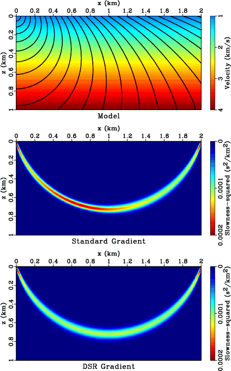
According to equations 11 and 15, the sensitivity
kernels (a row of Frechét derivative matrix) of standard tomography and DSR
tomography are different. Figure 10 compares sensitivity kernels for the same
source-receiver pair in a constant velocity-gradient model. We use a fine model sampling of
![]() m. The standard tomography kernel appears to be asymmetric. Its amplitude has a bias
towards the source side, while the width is broader on the receiver side. These phenomena are related to our
implementation, as described in Appendix C. Note in the top plot of Figure 10, the curvature of
first-break wave-front changes during propagation. Upwind finite-differences
take the curvature variation into consideration and, as a result, back-project
data-misfit with different weights along the ray-path. Meanwhile, the DSR tomography kernel is symmetric in both
amplitude and width, even though it uses the same discretization and upwind approximation as
in standard tomography. The source-receiver reciprocity may suggest averaging the standard tomography kernel with
its own mirroring around
m. The standard tomography kernel appears to be asymmetric. Its amplitude has a bias
towards the source side, while the width is broader on the receiver side. These phenomena are related to our
implementation, as described in Appendix C. Note in the top plot of Figure 10, the curvature of
first-break wave-front changes during propagation. Upwind finite-differences
take the curvature variation into consideration and, as a result, back-project
data-misfit with different weights along the ray-path. Meanwhile, the DSR tomography kernel is symmetric in both
amplitude and width, even though it uses the same discretization and upwind approximation as
in standard tomography. The source-receiver reciprocity may suggest averaging the standard tomography kernel with
its own mirroring around ![]() km, however the result will still be different from the DSR tomography kernel as
the latter takes into consideration all sources at the same time.
km, however the result will still be different from the DSR tomography kernel as
the latter takes into consideration all sources at the same time.
|
|---|
|
grad
Figure 10. (Top) model overlaid with traveltime contours of a source at |
|
|
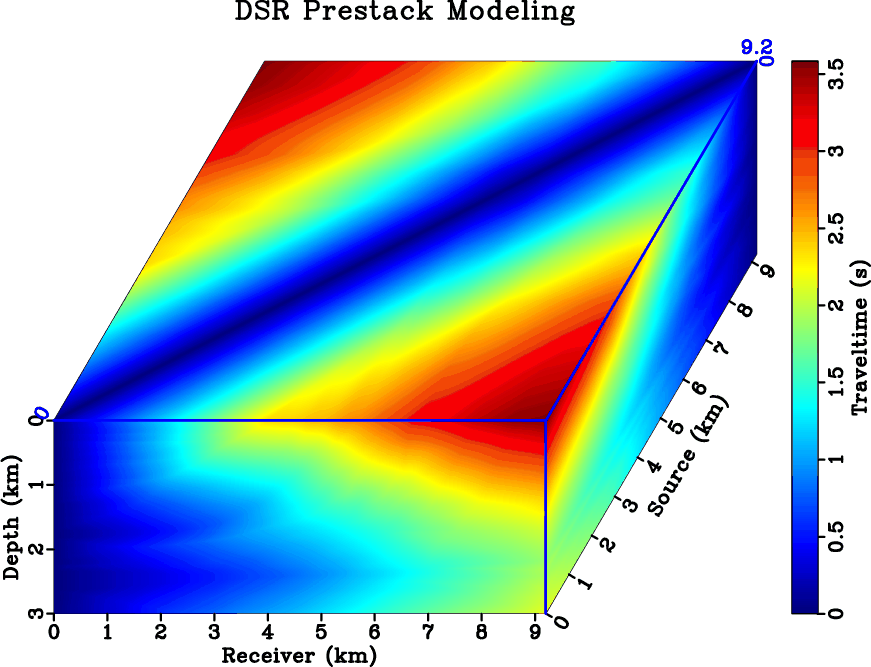
Finally, Figure 11 illustrates a prestack first-break traveltime modeling of the Marmousi model by
DSR FMM. We use a constant-velocity-gradient model as the prior for inversion. There are ![]() shots evenly distributed on the surface, each shot has a maximum absolute receiver offset of
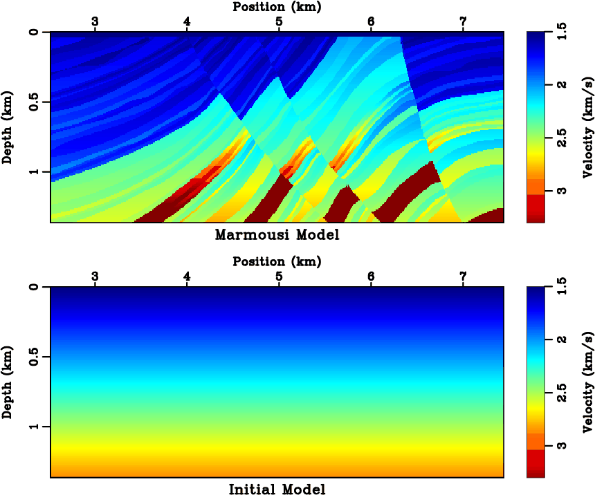
shots evenly distributed on the surface, each shot has a maximum absolute receiver offset of ![]() km. Figure 12 shows a zoom-in of the exact model that is within the tomographic aperture. The DSR
tomography and standard tomography are performed with the same parameters:
km. Figure 12 shows a zoom-in of the exact model that is within the tomographic aperture. The DSR
tomography and standard tomography are performed with the same parameters: ![]() conjugate gradient iterations per
linearization update and
conjugate gradient iterations per
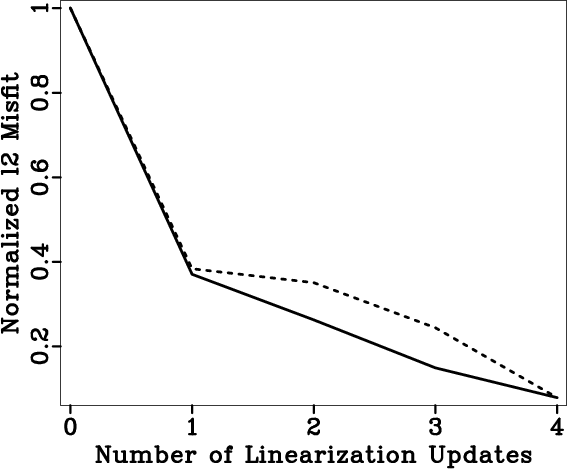
linearization update and ![]() linearization updates in total. Figure 13 shows the convergence
histories. While both inversions converge, the relative
linearization updates in total. Figure 13 shows the convergence
histories. While both inversions converge, the relative ![]() data misfits of DSR tomography decreases faster
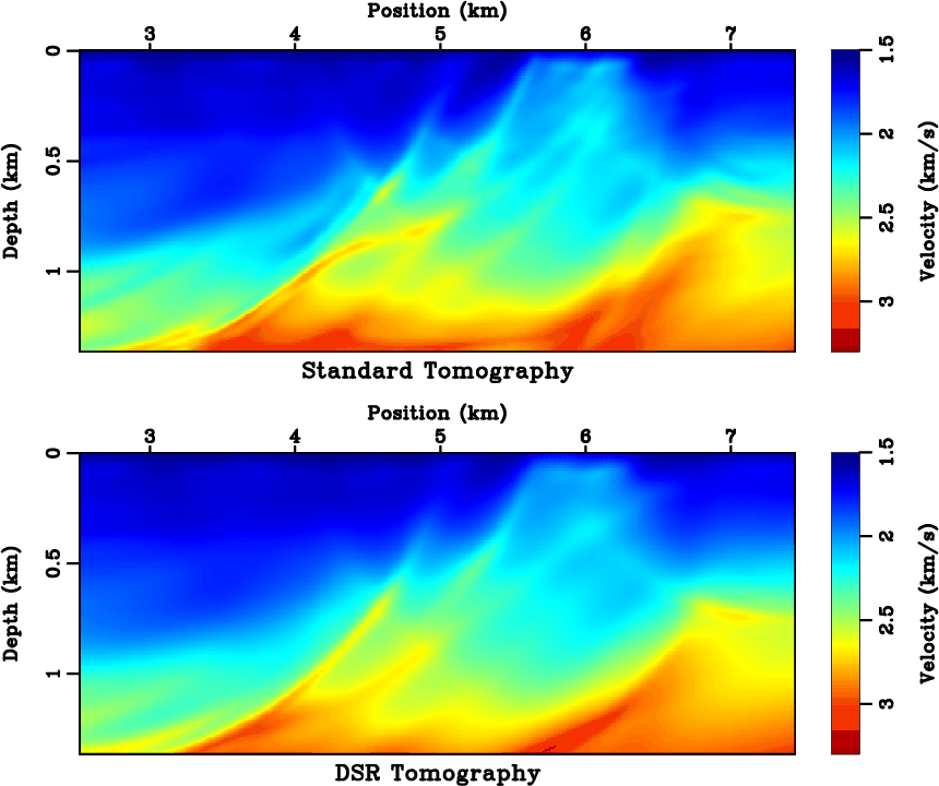
than that of standard tomography. Figure 14 compares the recovered models. Although both results
resemble the exact model in Figure 12 at the large scale, the standard tomography model exhibits
several undesired structures. For example, a near-horizontal structure with a velocity of around
data misfits of DSR tomography decreases faster
than that of standard tomography. Figure 14 compares the recovered models. Although both results
resemble the exact model in Figure 12 at the large scale, the standard tomography model exhibits
several undesired structures. For example, a near-horizontal structure with a velocity of around ![]() km/s at
location
km/s at
location ![]() km is false. It indicates the presence of a local minimum that has trapped the standard
tomography. In practice, it is helpful to tune the inversion parameters so that the standard tomography takes
more iterations with a gradually reducing regularization. The inversion parameters are usually empirical and hard
to control. Our analysis in preceeding sections suggests that part of the role of regularization is to deal with
conflicting information between shots. In contrast, we find DSR tomography less dependent on regularization and
hence more robust.
km is false. It indicates the presence of a local minimum that has trapped the standard
tomography. In practice, it is helpful to tune the inversion parameters so that the standard tomography takes
more iterations with a gradually reducing regularization. The inversion parameters are usually empirical and hard
to control. Our analysis in preceeding sections suggests that part of the role of regularization is to deal with
conflicting information between shots. In contrast, we find DSR tomography less dependent on regularization and
hence more robust.
|
|---|
|
data
Figure 11. DSR first-break traveltimes in the Marmousi model. The original model is decimated by |
|
|
|
|---|
|
marm
Figure 12. (Top) a zoom-in of Marmousi model and (bottom) the initial model for tomography. |
|
|
|
|---|
|
conv
Figure 13. Convergency history of DSR tomography (solid) and standard tomography (dashed). There is no noticeable improvement on misfit after the fourth update. |
|
|
|
|---|
|
tomo
Figure 14. Inverted model of (top) standard tomography and (bottom) DSR tomography. Compare with Figure 12. |
|
|
The advantage of DSR tomography becomes more significant in the presence of
noise in the input data. We generate random noise of normal distribution with zero mean and a
range between ![]() ms, then threshold the result with a minimum absolute value of
ms, then threshold the result with a minimum absolute value of ![]() ms. This is to mimic
the spiky errors in first-breaks estimated from an automatic picker. After adding noise to the data, we run
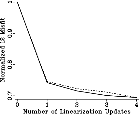
inversions with the same parameters as in Figures 13 and 14. Figures 15 and
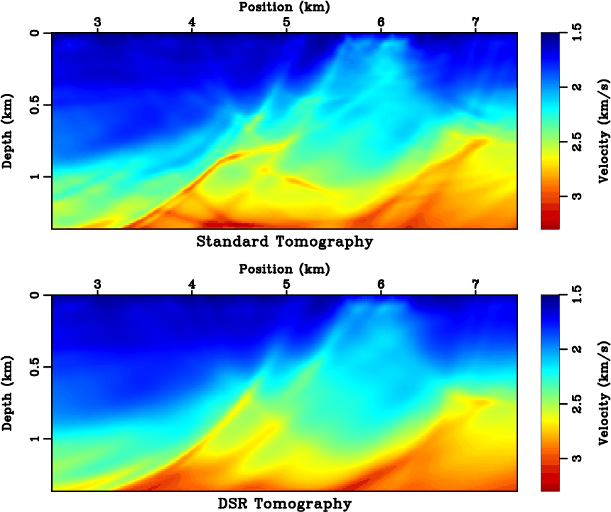
16 show the convergence history and inverted models. Again, the standard tomography seems to provide
a model with higher resolution, but a close examination reveals that many small scale details are in fact
non-physical. On the other hand, DSR tomography suffers much less from the added noise. Adopting a
ms. This is to mimic
the spiky errors in first-breaks estimated from an automatic picker. After adding noise to the data, we run
inversions with the same parameters as in Figures 13 and 14. Figures 15 and
16 show the convergence history and inverted models. Again, the standard tomography seems to provide
a model with higher resolution, but a close examination reveals that many small scale details are in fact
non-physical. On the other hand, DSR tomography suffers much less from the added noise. Adopting a ![]() norm in objective function 5 can improve the inversion, especially for standard tomography.
However, it also raises the difficulty in selecting appropriate inversion
parameters.
norm in objective function 5 can improve the inversion, especially for standard tomography.
However, it also raises the difficulty in selecting appropriate inversion
parameters.
|
|---|
|
nconv
Figure 15. Inversion with noisy data. Convergency history of DSR tomography (solid) and standard tomography (dashed). No significant decrese in misfit appears after the fourth update. |
|
|
|
|---|
|
ntomo
Figure 16. Inversion with noisy data. Inverted model of (top) standard tomography and (bottom) DSR tomography. Compare with Figure 14. |
|
|
|
|
|
|
First-break traveltime tomography with the double-square-root eikonal equation |