From modeling to full waveform inversion: A hands-on tour using Madagascar

Do a synthetic FWI test using Marmousi model

It is convenient to perform adjoint simulation when reconstructing the incident wavefield backwards. The computation of FWI gradient can be done on the fly by adding several lines: Of course, to apply the steepest descent method for minimization of the misfit function for waveform inversion, a step length has to be determined at each iteration. You may use the estimation proposed by Pica et al. (1990, in the appendix) in your FWI code as RSFSRC/user/pyang/Mfwi2d.c.

The workflow for synthetic FWI test based on Marmousi model follows the several steps:

1. Obtain the Marmousi velocity model, which can be downloaded by Fetch('marmvel.hh','marm') in SConstruct, as shown in the top panel of Figure 4.

2. We may start to generate the observed seismograms/shots using resampled Marmousi, as shown in Figure 5.

3. By smoothing the true model using triangular window many times, an initial model plotted in the bottom panel of Figure 4 is generated to do the FWI test.

4. Using the observed seismograms/shots from true model, we start the inversion with the rough initial model.

5. You may appreciate your the inverted velocity during the iterations in Figure 6, as well as the variations of the misfit function in Figure 7.

A complete SConstruct for the above workflow appears in the following:

from rsf.proj import *

# marmvel.hh contains Marmousi model which can
# be downloaded from the server using Fetch.
Fetch('marmvel.hh','marm')

Flow('vel','marmvel.hh',
	'''
	dd form=native | window j1=8 j2=8 | sfsmooth rect1=3 rect2=3|
     	put label1=Depth  unit1=m label2=Lateral unit2=m
	''')
Plot('vel',
	'''
	grey color=j mean=y title="Marmousi model" 
	scalebar=y bartype=v barlabel="V" 
	barunit="m/s" screenratio=0.45 color=j labelsz=10 titlesz=12
	''')

Flow('shots','vel',
	'''
	sfmodeling2d csdgather=n fm=4 amp=1 dt=0.0015 ns=7 ng=288 nt=2800
	sxbeg=4 szbeg=2 jsx=45 jsz=0 gxbeg=0 gzbeg=3 jgx=1 jgz=0
	''')
Plot('shots','grey color=g title=shot label2= unit2=',view=1)

Plot('shot1','shots',
     'window n3=1 f3=0| grey title=shot1 label2=Lateral unit2=m')
Plot('shot3','shots',
     'window n3=1 f3=2| grey title=shot3 label2=Lateral unit2=m')
Plot('shot5','shots',
     'window n3=1 f3=4| grey title=shot5 label2=Lateral unit2=m')
Plot('shot7','shots',
     'window n3=1 f3=6| grey title=shot7 label2=Lateral unit2=m')
Result('shotsnap','shot1 shot3 shot5 shot7',
       'SideBySideAniso',vppen='txscale=2.')

# smoothed velocity model   
Flow('smvel','vel','smooth repeat=6  rect1=8 rect2=10')
Plot('smvel',
     '''
     grey title="Initial model" wantitle=y allpos=y color=j
     pclip=100 scalebar=y bartype=v barlabel="V" barunit="m/s"
	 screenratio=0.45 color=j labelsz=10 titlesz=12
     ''' )

Result('marm','vel smvel','TwoRows')

# use the over-smoothed model as initial model for FWI
Flow('vsnaps grads objs illums','smvel shots',
	'''
	sffwi2d shots=${SOURCES[1]} 
        grads=${TARGETS[1]} objs=${TARGETS[2]}
	illums=${TARGETS[3]} niter=10 precon=y rbell=1
	''')
Result('vsnaps',
	'''
	grey title="Updated velocity" allpos=y color=j pclip=100 
	scalebar=y bartype=v barlabel="V" barunit="m/s" 
	''')
Plot('vsnap1','vsnaps', 
	'''
	window n3=1|grey title="Updated velocity, iter=1" 
	allpos=y color=j pclip=100 labelsz=10 titlesz=12
	scalebar=y bartype=v barlabel="V" barunit="m/s" 
	''')
Plot('vsnap2','vsnaps', 
	'''
	window n3=1 f3=1|grey title="Updated velocity, iter=2" 
	allpos=y color=j pclip=100 labelsz=10 titlesz=12
	scalebar=y bartype=v barlabel="V" barunit="m/s" 
	''')
Plot('vsnap4','vsnaps', 
	'''
	window n3=1 f3=3|grey title="Updated velocity, iter=4" 
	allpos=y color=j pclip=100 labelsz=10 titlesz=12
	scalebar=y bartype=v barlabel="V" barunit="m/s" 
	''')

Plot('vsnap6','vsnaps', 
	'''
	window n3=1 f3=5|grey title="Updated velocity, iter=6"
	 allpos=y color=j pclip=100 labelsz=10 titlesz=12
	scalebar=y bartype=v barlabel="V" barunit="m/s" 
	''')
Plot('vsnap8','vsnaps', 
	'''
	window n3=1 f3=7|grey title="Updated velocity, iter=8"
	allpos=y color=j pclip=100 labelsz=10 titlesz=12
	scalebar=y bartype=v barlabel="V" barunit="m/s" 
	''')
Plot('vsnap10','vsnaps', 
	'''
	window n3=1 f3=9|grey title="Updated velocity, iter=10" 
	allpos=y color=j pclip=100 labelsz=10 titlesz=12
	scalebar=y bartype=v barlabel="V" barunit="m/s" 
	''')

Result('vsnap','vsnap1 vsnap2 vsnap4 vsnap6 vsnap8 vsnap10',
       'TwoRows')

Result('objs',
	'''
	sfput n2=1 label1=Iteration unit1= unit2= label2= |
	graph title="Misfit function" dash=0 plotfat=5 
        grid=y yreverse=n
	''')

End()

marm
Figure 4. Top: True Marmousi model; bottom: Initial model for FWI

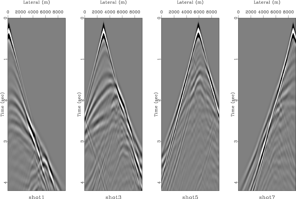
shotsnap
Figure 5. Shots from true Marmousi model

vsnap
Figure 6. Inverted velocity during iterations

objs
Figure 7. The misfit function decreases during iterations

From modeling to full waveform inversion: A hands-on tour using Madagascar