|
|
|
|
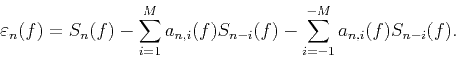
Random noise attenuation using |
Nonstationary autoregression has been developed and used in signal processing
(AllenAboutajdine et al., 1996; Bakrim et al., 1994; Izquierdo et al., 2006) and seismic data processing
(Sacchi and Naghizadeh, 2009). Fomel (2009) developed a general method of nonstationary
autoregression using shaping regularization technology and applied it to multiples
subtraction. In this paper, we extend the RNA method to ![]() -
-![]() domain for complex numbers
and apply it to seismic random noise attenuation.
domain for complex numbers
and apply it to seismic random noise attenuation.
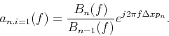
Consider two adjacent seismic traces ![]() and
and
![]() in
in
![]() -
-![]() domain of a seismic section that consists of a single nonlinear event with the
slope
domain of a seismic section that consists of a single nonlinear event with the
slope ![]() and varying amplitude
and varying amplitude ![]() . Similar to equation 1,
we can write
. Similar to equation 1,
we can write
From equation 5 we can find that the coefficients of AR is the function of space index
![]() and frequency index
and frequency index ![]() . Therefore, we can use nonstationary autoregression to
describe this problem. Equation 5 describes the relation between two traces.
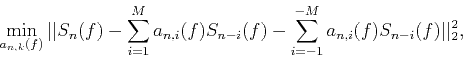
If we consider multiple traces, the nonstationary autoregression can be defined as (Fomel, 2009)
. Therefore, we can use nonstationary autoregression to
describe this problem. Equation 5 describes the relation between two traces.
If we consider multiple traces, the nonstationary autoregression can be defined as (Fomel, 2009)
The problem of the minimization in equation 7 is ill-posed because it has more unknown variables than constraints. To obtain the spatial-varying coefficients in nonstationary autoregression, several methods can be employed (AllenAboutajdine et al., 1996). Some of these are related to the expansion of the spatial-varying coefficients in terms of a given sets of orthogonal basis functions and estimation of the coefficients of the expansion by the least-square method (Izquierdo et al., 2006). Naghizadeh and Sacchi (2009) used exponentially weighted recursive least square (EWRLS) to solve the adaptive problem and applied it to seismic trace interpolation. Fomel (2009) proposed regularized nonstationary autoregression in which shaping regularization technology (Fomel, 2007) is used to constrain the smoothness of the coefficients of nonstationary autoregression. In this paper, we also adopt shaping regularization to solve the under-constrained problem equation 8.
With the addition of a regularization term, equation 8 can be written as
Note that the RNA equation in this paper (equation 9) is in complex
number domain while the RNA used in multiples subtraction (Fomel, 2009)
is in real number domain. Analogous to RNA in real number domain,
we force the complex coefficients
![]() in equation 9
to have a desired behavior, such as smoothness. In shaping regularization technology,
we need to choose a shaping operator
in equation 9
to have a desired behavior, such as smoothness. In shaping regularization technology,
we need to choose a shaping operator ![]() (Fomel, 2007).
In this paper, we choose shaping operator
(Fomel, 2007).
In this paper, we choose shaping operator ![]() as Gaussian smoothing with adjustable radius
as Gaussian smoothing with adjustable radius ![]() .
Fomel (2007) indicated Gaussian smoothing can be implemented by repeated triangle smoothing operator.
Both the data
.
Fomel (2007) indicated Gaussian smoothing can be implemented by repeated triangle smoothing operator.
Both the data ![]() and the coefficients
and the coefficients
![]() are complex numbers, but the shaping
operator
are complex numbers, but the shaping
operator ![]() is real. Therefore, shaping operator
is real. Therefore, shaping operator ![]() is operated in real and imaginary
parts of the complex coefficients respectively and the L-2 norm in equation 9 is the norm of complex numbers.
When using the algorithm of conjugate-gradient iterative inversion with shaping regularization proposed by Fomel (2007)
to solve the complex RNA, we only need to replace transpose of real number by conjugate transpose of complex number.
is operated in real and imaginary
parts of the complex coefficients respectively and the L-2 norm in equation 9 is the norm of complex numbers.
When using the algorithm of conjugate-gradient iterative inversion with shaping regularization proposed by Fomel (2007)
to solve the complex RNA, we only need to replace transpose of real number by conjugate transpose of complex number.
Once we obtain the complex coefficients of RNA, we can achieve an estimation of signal
The computational cost of the proposed method is
![]() ,
where
,
where ![]() is data size,
is data size, ![]() is filter size,
is filter size, ![]() is the number of
conjugate-gradient iterations. If
is the number of
conjugate-gradient iterations. If ![]() and
and ![]() are small, this is a
fast method. In practical implementation, we can choose the range of computed
frequency to reduce the computation cost. In addition, if we can simplify the
coefficients not to be frequency-dependent, we can apply RNA in frequency slice.
In that case the different-frequency slices can be processed in parallel.
And the computation cost and memory requirements can be further reduced.
are small, this is a
fast method. In practical implementation, we can choose the range of computed
frequency to reduce the computation cost. In addition, if we can simplify the
coefficients not to be frequency-dependent, we can apply RNA in frequency slice.
In that case the different-frequency slices can be processed in parallel.
And the computation cost and memory requirements can be further reduced.


|
|---|
|
sin,nsin,tpefpatch,fxpatch,npre1,npre2
Figure 1. (a) Synthetic data. (b) Noisy data (SNR=1.53). (c) Result of |
|
|

|
|---|
|
npar2
Figure 2. The real part of coefficients at a given shift |
|
|


|
|---|
|
fxdiff,mpapatch,ndiff2
Figure 3. Difference sections of |
|
|
Consider a simple section (Figure 1(a)), which includes one event, 501 traces.
The event is obtained by convolution with Ricker wavelet. Both the dip and amplitude
of the event are space-varying. The travel time is a sine function and the amplitude of
the Ricker wavelet is multiplied by
![]() . This event is obviously
nonstationary in space. We add some random noise to it (Figure 1(b)).
The event is greatly contaminated by random noise, especially in the middle part,
because the signal of the middle part is poorer than the sideward and the noise levels
are the same in the whole section. We use three methods,
. This event is obviously
nonstationary in space. We add some random noise to it (Figure 1(b)).
The event is greatly contaminated by random noise, especially in the middle part,
because the signal of the middle part is poorer than the sideward and the noise levels
are the same in the whole section. We use three methods, ![]() -
-![]() domain prediction,
domain prediction, ![]() -
-![]() domain prediction, and
domain prediction, and ![]() -
-![]() domain RNA, to suppress random noise. The
domain RNA, to suppress random noise. The ![]() -
-![]() domain and
domain and ![]() -
-![]() domain prediction methods we used in this paper are discussed by (Abma and Claerbout, 1995).
The
domain prediction methods we used in this paper are discussed by (Abma and Claerbout, 1995).
The ![]() -
-![]() domain prediction is implemented over a sliding window of 20 traces width with 50%
overlap and the filter length is 4,
domain prediction is implemented over a sliding window of 20 traces width with 50%
overlap and the filter length is 4, ![]() in equation 4 and the
in equation 4 and the ![]() -
-![]() domain prediction is
implemented over the same sliding window and the filter length in space and time are 4 and 5
respectively. The
domain prediction is
implemented over the same sliding window and the filter length in space and time are 4 and 5
respectively. The ![]() -
-![]() RNA is implemented with the parameters: the filter length is 4,
RNA is implemented with the parameters: the filter length is 4, ![]() in equation 8; the smoothing radiuses in space and frequency axes of shaping regularization are
respectively 20 and 3,
in equation 8; the smoothing radiuses in space and frequency axes of shaping regularization are
respectively 20 and 3, ![]() ,
, ![]() . Comparing the results of
. Comparing the results of ![]() -
-![]() RNA (Figure 1(f))
with other prediction methods (Figures 4(c) and 4(d), we find that the
RNA (Figure 1(f))
with other prediction methods (Figures 4(c) and 4(d), we find that the
![]() -
-![]() RNA is more effective in random noise attenuation for this simple nonstationary data. From the
difference sections (Figure 2), we find that all the three methods remove
some effective signals. However, the proposed method removes fewest signals than other two methods.
Note that the removed signals by
RNA is more effective in random noise attenuation for this simple nonstationary data. From the
difference sections (Figure 2), we find that all the three methods remove
some effective signals. However, the proposed method removes fewest signals than other two methods.
Note that the removed signals by ![]() -
-![]() and
and ![]() -
-![]() prediction methods are bigger in the sideward
part than middle part, because the filters are the same in a sliding time window while
the amplitude and slope of the event are different.
prediction methods are bigger in the sideward
part than middle part, because the filters are the same in a sliding time window while
the amplitude and slope of the event are different.
In order to quantitatively evaluate the effect of denoising between different methods,
we use signal-to-noise ratio (SNR) to compare these three methods. The SNR is estimated by
To test the sensitivity to the constraint of smoothness along the frequency axis, we give the result of ![]() -
-![]() RNA without constraint of smoothness along the frequency axis in this simple example (Figure 1(e)). The result without constraint along frequency axis
(Figure 1(e)) is a little worse than that with constraint along frequency.
But both of them are better than the results of conventional
RNA without constraint of smoothness along the frequency axis in this simple example (Figure 1(e)). The result without constraint along frequency axis
(Figure 1(e)) is a little worse than that with constraint along frequency.
But both of them are better than the results of conventional ![]() -
-![]() domain and
domain and ![]() -
-![]() domain prediction.
Therefore, to reduce the computation cost, we can simplify the coefficients not to be frequency-dependent
when the input seismic data is huge. It is a tradeoff between computation cost and effect of noise attenuation.
domain prediction.
Therefore, to reduce the computation cost, we can simplify the coefficients not to be frequency-dependent
when the input seismic data is huge. It is a tradeoff between computation cost and effect of noise attenuation.
Because the dip and amplitude of the event are varying smoothly, ![]() -
-![]() RNA can predict the signal with smooth
coefficients
RNA can predict the signal with smooth
coefficients
![]() . To specify the coefficients, we display the real parts of the complex
coefficients at a given shift
. To specify the coefficients, we display the real parts of the complex
coefficients at a given shift
![]() (Figure 2). The reason of displaying real parts not
imaginary parts is that the signs of real parts of coefficients are the same for forward and
backward prediction. We find that the real parts of the complex coefficients are smooth.
The smoothing radius controls the smoothness of the coefficients. If we only use one adjacent
trace to predict the trace, the coefficients should have the expression
(Figure 2). The reason of displaying real parts not
imaginary parts is that the signs of real parts of coefficients are the same for forward and
backward prediction. We find that the real parts of the complex coefficients are smooth.
The smoothing radius controls the smoothness of the coefficients. If we only use one adjacent
trace to predict the trace, the coefficients should have the expression
|
|
|
|
Random noise attenuation using |


![\begin{displaymath}
\min_{a_{n,i}{f}}\vert\vert{{S}_{n}}(f)-\sum\limits_{i=-M,i...
...i}}(f){{S}_{n-i}}(f)}\vert\vert _{2}^{2}+R[{{a}_{n,i}}(f)],
\end{displaymath}](img32.png)

![\begin{displaymath}
SNR=10{{\log }_{10}}(\frac{\sum\limits_{t,n}{{{[{{d}_{n}}(t...
...}{\sum\limits_{t,n}{{{[{{d}_{n}}(t)-{{r}_{n}}(t)]}^{2}}}}),
\end{displaymath}](img45.png)