Numeric implementation of wave-equation migration velocity analysis operators

Examples

zokernel
Figure 1. Schematic representation of the forward and adjoint operators for ray-based MVA and wave-based MVA. The forward operator $F$ applied to a slowness anomaly $\Delta s$ generates a traveltime perturbation (a) or an image perturbation (b). The ray-based adjoint MVA operator $A$ applied to the traveltime perturbation generates a slowness perturbation uniformly distributed along a ray normal to the reflector (c). The wave-based adjoint MVA operator $A$ applied to the image perturbation generates a slowness perturbation with a wider space distribution but with a relative focus at the location of the original slowness anomaly (d).

We illustrate the wave-equation migration velocity analysis operators using impulse responses corresponding to different imaging configurations. We concentrate on imaging in the zero-offset and shot-record frameworks, since they also implicitly characterize the essential elements of the survey-sinking framework. In all cases, we use wavefield reconstruction based on one-way wavefield extrapolation with the multi-reference split-step Fourier method (Stoffa et al., 1990; Popovici, 1996).

vel,img
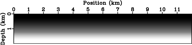
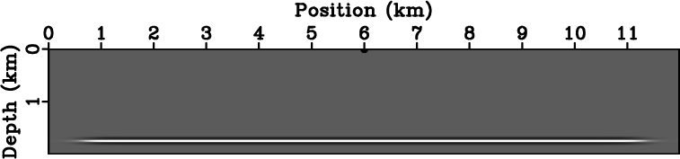
Figure 2. Simple synthetic model with (a) linear $v\left (z \right)$ velocity and (b) a horizontal reflector.

A fundamental question concerning the wavefield scattering operator ( ${\textbf{\sc w.s.}}$) is what is its sensitivity for a given perturbation of the image or of the slowness model. This sensitivity is usually characterized using the so-called ``sensitivity kernels'' which are often discussed in the literature in the context of tomography problems. For wave-equation MVA, this topic was discussed in the context of zero-offset imaging by Sava and Biondi (2004a,b). The important topic of sensitivity and model resolution falls outside the scope of this paper, so we do not discuss it here in any detail. We merely concern ourselves with describing the behavior of the wave-equation MVA operators described earlier.

ds4,di4
Figure 3. (a) Slowness perturbations used to demonstrate the WEMVA operators in Figures 5(a)-6(b), and (b) image perturbation used to demonstrate the WEMVA operators in Figures 7(a)-8(b).

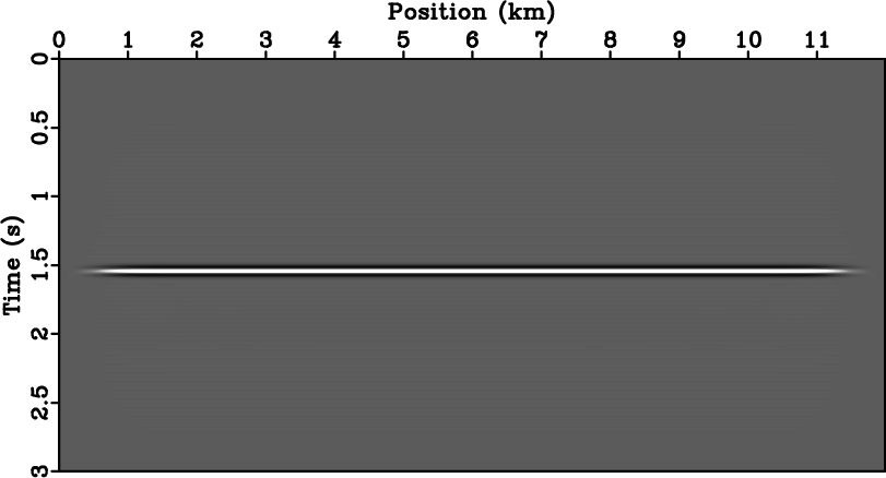
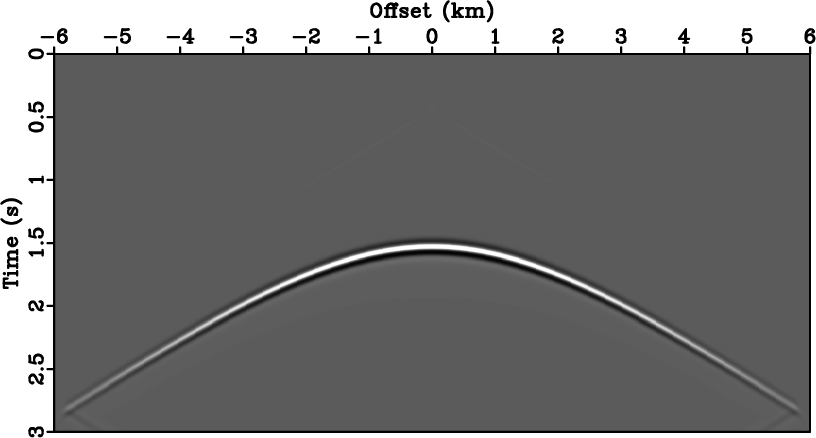
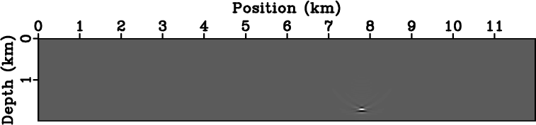
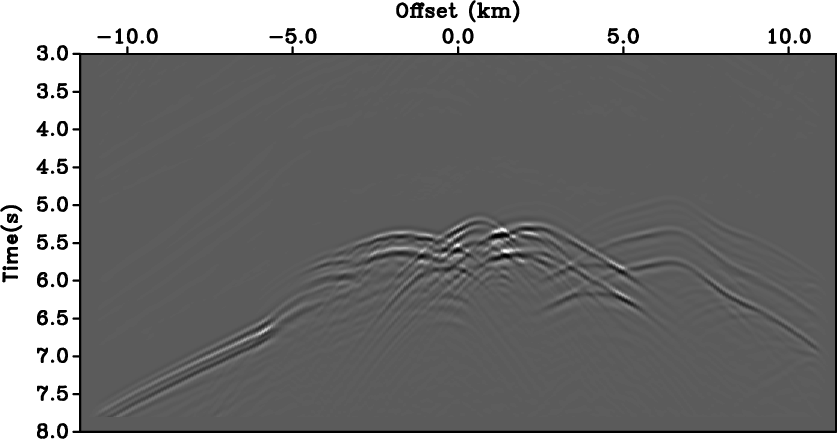
Zdat,Sdat
Figure 4. (a) Simulated zero-offset data and (b) simulated shot-record data for the model depicted in Figures 2(a)-2(b) with a source located at coordinates $x=6$ km and $z=0$ km.

We can analyze the sensitivity of the wavefield scattering operator in two ways. The first option is to assume a localized slowness perturbation, compute image perturbations using the forward scattering operator and then return to the slowness perturbation using the adjoint scattering operator. The second option is to assume a localized image perturbation, compute the slowness perturbation using the adjoint scattering operator and then return to the image perturbation using the forward scattering operator.

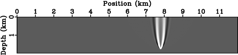
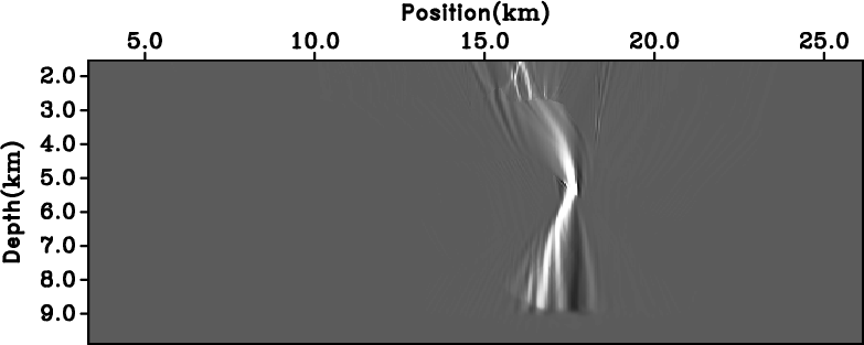
ZFds4,ZAFds4
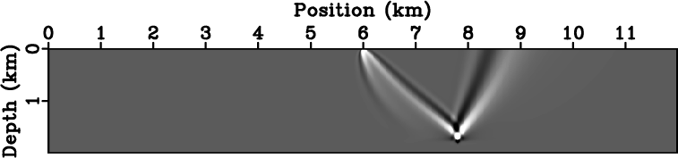
Figure 5. (a) Zero-offset image perturbation obtained by the application of the forward scattering operator to the slowness perturbation from Figure 3(a) and (b) zero-offset slowness perturbation obtained by the application of the adjoint scattering operator to the image perturbation from panel (a).

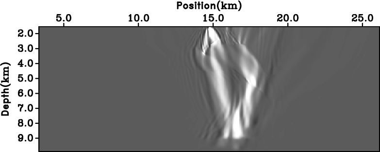
SFds4,SAFds4
Figure 6. (a) Shot-record image perturbation obtained by the application of the forward scattering operator to the slowness perturbation from Figure 3(a) and (b) shot-record slowness perturbation obtained by the application of the adjoint scattering operator to the image perturbation from panel (a).

As discussed in the preceding sections, the main difference between ray-based and wave-based MVA techniques is that the connection between measurements on the image and updates to the model is done with rays and waves, respectively. The impact of this fundamental difference is best seen if we analyze impulse responses of the wave-equation MVA and compare them with those of conventional traveltime tomography. Figure 1 shows a one-to-one comparison between the forward and adjoint operators for ray-based MVA (traveltime tomography) on the left and wave-based MVA on the right in the context of zero-offset imaging. Assuming a small slowness perturbation $\Delta s$, we can construct using the forward MVA operators a traveltime perturbation and an image perturbation corresponding to ray-based MVA (a) and wave-based MVA (b), respectively. For this zero-offset configuration, the ray-based MVA produces a traveltime anomaly strictly located on the reflector under the slowness anomaly, while the wave-based MVA produces an image anomaly distributed in space in the vicinity of the reflector. Then, we can construct respective slowness updates if we apply the ray-based and wave-based adjoint MVA operators to the traveltime perturbation and image perturbation, respectively. For the ray-based MVA, the slowness update spreads uniformly along a ray orthogonal to the reflector (c), while for wave-based MVA, the slowness update is distributed in space from the image perturbation to the surface, but with a concentration at the location of the true anomaly (d). Similar behavior characterizes wave-equation MVA under shot-record or survey-sinking frameworks.

ZAdi4,ZFAdi4
Figure 7. (a) Zero-offset slowness perturbation obtained by the application of the adjoint scattering operator to the image perturbation from Figure 3(b) and (b) zero-offset image perturbation obtained by the application of the forward scattering operator to the slowness perturbation from panel (a).

SAdi4,SFAdi4
Figure 8. (a) Shot-record slowness perturbation obtained by the application of the adjoint scattering operator to the image perturbation from Figure 3(a) and (b) shot-record image perturbation obtained by the application of the forward scattering operator to the slowness perturbation from panel (a).

The first set of examples corresponds to a simple model consisting of a linear $v\left (z \right)$ velocity model and a horizontal reflector, Figures 2(a)-2(b). The velocity is linearly increasing from $1.5$ km/s to $2.75$ km/s. We simulate zero-offset data, Figure 4(a), and one shot corresponding to horizontal position $x=6$ km, Figure 4(b).

Assuming a localized slowness perturbation, Figure 3(a), we can compute image perturbations using the forward scattering operators, as defined in the preceding sections. Figure 5(a) shows the image perturbation for the zero-offset case and Figure 6(a) shows the similar image perturbation for the shot-record case. As illustrated in Figure 1, the image perturbations are distributed in the vicinity of the reflector. Two interfering events are seen for the shot-record case, corresponding to the source and receiver wavefields, respectively.

Similarly, we can compute slowness perturbations using the adjoint scattering operators. Figure 5(b) shows the slowness perturbation for the zero-offset case computed from the image perturbation in Figure 5(a) and Figure 6(b) shows the similar slowness perturbation for the shot-record case computed from the image perturbation in Figure 6(a). As illustrated in Figure 1, the slowness perturbations are distributed in an area connecting the reflector to the surface, but with a relative focus at the location of the original anomaly. For the shot-record case, the back-projection splits toward the source and receivers, corresponding to the upward continuation of the source and receiver wavefields.

We can also analyze the wave-equation MVA operator sensitivity in another way. Assuming a localized image perturbation, Figure 3(b), we can compute slowness perturbations using the adjoint scattering operators, as defined in the preceding sections. Figure 7(a) shows the slowness perturbation for the zero-offset case and Figure 8(a) shows the similar slowness perturbation for the shot-record case. Here, too, we see slowness perturbations distributed in an area connecting the reflector to the surface, but in this case, there is no relative focus of the anomaly because the image perturbation is strictly localized on the reflector. For the shot-record case, the back-projection splits toward the source and receivers, corresponding to the upward continuation of the source and receiver wavefields. This case corresponds to the case of practical MVA where measurements of defocusing features are made on the image itself.

As we have done in the preceding experiment, we can also compute image perturbations using the forward scattering operators based on the back-projections created using the adjoint scattering operators. Figure 7(b) shows the image perturbation for the zero-offset case computed from the slowness perturbation in Figure 7(a) and Figure 8(b) shows the similar image perturbation for the shot-record case computed from the slowness perturbation in Figure 8(a). We can observe that the resulting image perturbations spread beyond the original location, indicating wider sensitivity of the wave-based MVA kernels to image perturbations than that of the corresponding ray-based MVA kernels.

Similar sensitivity can be observed for the more complex Sigsbee 2A model (Paffenholz et al., 2002), Figures 9(a)-9(b). Similarly to the preceding example, we simulate zero-offset data, Figure 11(a), and one shot corresponding to horizontal position $x=14.6$ km, Figure 11(b).

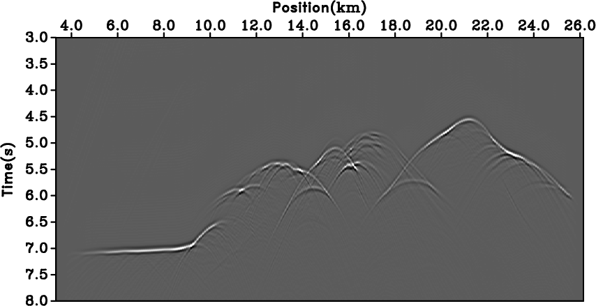
Figures 12(a) and 13(a) correspond to the image perturbations for the slowness anomaly shown in Figure 10(a). We can observe image perturbations that spread in the vicinity of the reflector, similarly to the simpler example described earlier. The multi-pathing from the source to the reflector generates the multiple events characterizing the image perturbations. Figures 12(b) and 13(b) correspond to the slowness perturbations constructed by applying the zero-offset and shot-record adjoint scattering operators to the image perturbations from Figures 12(a) and 13(a). We see similar back-projection patterns to the ones observed in the preceding example, except that the propagation pattens are more complicated due to the presence of the salt body in the background model.

Figures 14(a) and 15(a) correspond to the slowness perturbations for the image anomaly shown in Figure 10(b). We can observe slowness perturbations that spread in the vicinity of the reflector, similarly to the simpler example described earlier. Finally, Figures 14(b) and 15(b) correspond to the image perturbations for the slowness perturbations constructed by the adjoint MVA operators shown in Figures 14(a) and 15(a) for the zero-offset and shot-record cases, respectively.

vel,img
Figure 9. (a) Sigsbee 2A synthetic model and (b) a sub-salt horizontal reflector.

ds2,di2
Figure 10. (a) Slowness perturbations used to demonstrate the WEMVA operators in Figures 12(a)-13(b), and (b) image perturbation used to demonstrate the WEMVA operators in Figures 14(a)-15(b).

Zdat,Sdat
Figure 11. (a) Simulated zero-offset data and (b) simulated shot-record data for the model depicted in Figures 9(a)-9(b) with a source located at coordinates $x=14.6$ km and $z=1.52$ km.

ZFds2,ZAFds2
Figure 12. (a) Zero-offset image perturbation obtained by the application of the forward scattering operator to the slowness perturbation from Figure 10(a) and (b) zero-offset slowness perturbation obtained by the application of the adjoint scattering operator to the image perturbation from panel (a).

SFds2,SAFds2
Figure 13. (a) Shot-record image perturbation obtained by the application of the forward scattering operator to the slowness perturbation from Figure 10(a) and (b) shot-record slowness perturbation obtained by the application of the adjoint scattering operator to the image perturbation from panel (a).

ZAdi2,ZFAdi2
Figure 14. (a) Zero-offset slowness perturbation obtained by the application of the adjoint scattering operator to the image perturbation from Figure 10(b) and (b) zero-offset image perturbation obtained by the application of the forward scattering operator to the slowness perturbation from panel (a).

SAdi2,SFAdi2
Figure 15. (a) Shot-record slowness perturbation obtained by the application of the adjoint scattering operator to the image perturbation from Figure 10(a) and (b) shot-record image perturbation obtained by the application of the forward scattering operator to the slowness perturbation from panel (a).

Numeric implementation of wave-equation migration velocity analysis operators