|
|
|
|
Basic operators and adjoints |
The inverse of any polynomial reverberates forever, although it might
drop off fast enough for any practical need. On the other hand, a
rational filter can suddenly drop to zero and stay there. Let us look
at a popular rational filter, the rectangle or ``box car'':
| (30) |
	tmp2 = tmp + 2*nb;

	wt = 1.0/(2*nb-1);
	for (i=0; i < nx; i++) {
	    x[o+i*d] = (tmp[i+1] - tmp2[i])*wt;
	}
|
Triangle smoothing is rectangle smoothing done twice. For a mathematical description of the triangle filter, we simply square equation (29). Convolving a rectangle function with itself many times yields a result that mathematically tends toward a Gaussian function. Despite the sharp corner on the top of the triangle function, it has a shape remarkably similar to a Gaussian. Convolve a triangle with itself and you see a very nice approximation to a Gaussian (the central limit theorem).
With filtering, end effects can be a nuisance, especially on space axes. Filtering
increases the length of the data, but people generally want to keep
input and output the same length (for various practical reasons),
especially on a space axis. Suppose the
five-point signal ![]() is smoothed using the boxconv()
program with the three-point smoothing filter
is smoothed using the boxconv()
program with the three-point smoothing filter ![]() . The output
is
. The output
is ![]() points long, namely,
points long, namely,
![]() . We could simply
abandon the points off the ends, but I like to fold them back in,
getting instead
. We could simply
abandon the points off the ends, but I like to fold them back in,
getting instead
![]() . An advantage of the folding is
that a constant-valued signal is unchanged by the smoothing. Folding is
desirable because a smoothing filter is a low-pass filter that
naturally should pass the lowest frequency
. An advantage of the folding is
that a constant-valued signal is unchanged by the smoothing. Folding is
desirable because a smoothing filter is a low-pass filter that
naturally should pass the lowest frequency ![]() without
distortion. The result is like a wave reflected by a
zero-slope end condition. Impulses are smoothed
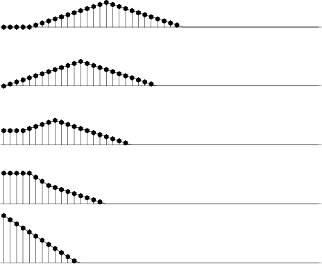
into triangles except near the boundaries. What happens near the
boundaries is shown in Figure 7.
without
distortion. The result is like a wave reflected by a
zero-slope end condition. Impulses are smoothed
into triangles except near the boundaries. What happens near the
boundaries is shown in Figure 7.
|
triend
Figure 7. Edge effects when smoothing an impulse with a triangle function. Inputs are spikes at various distances from the edge. |
|
|---|---|
|
|
Why this end treatment?
Consider a survey of water depth in an area of the deep ocean.
All the depths are strongly positive with interesting but small variations on them.
Ordinarily we can enhance high-frequency fluctuations by one minus a low-pass filter,
say ![]() . If this subtraction is to work, it is important
that the
. If this subtraction is to work, it is important
that the ![]() truly cancel the
truly cancel the ![]() near zero frequency.
near zero frequency.
Figure 7 was derived from the routine triangle().
	tmp1 = tmp + nb;
	tmp2 = tmp + 2*nb;

	wt = 1.0/(nb*nb);
	for (i=0; i < nx; i++) {
	    x[o+i*d] = (2.*tmp1[i] - tmp[i] - tmp2[i])*wt;
	}
|
|
|
|
|
Basic operators and adjoints |