 |
 |
 |
 | Model fitting by least squares |  |
![[pdf]](icons/pdf.png) |
Next: Estimating the inverse gradient
Up: Model fitting by least
Previous: Gulf of Mexico Salt
Figure 11 shows
radar images of
Mt. Vesuvius![[*]](icons/footnote.png) in Italy.
These images are made from backscatter
signals
in Italy.
These images are made from backscatter
signals  and
and  ,
recorded along two satellite orbits 800-km high and 54-m apart.
The signals are very high frequency
(the radar wavelength being 2.7 cm).
The signals were Fourier transformed
and one multiplied by the complex conjugate of the other,
getting the product
,
recorded along two satellite orbits 800-km high and 54-m apart.
The signals are very high frequency
(the radar wavelength being 2.7 cm).
The signals were Fourier transformed
and one multiplied by the complex conjugate of the other,
getting the product
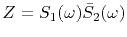 .
The product's amplitude and phase are shown in Figure 11.
Examining the data,
you can notice that where the signals are strongest (darkest on the left),
the phase (on the right)
is the most spatially consistent.
Pixel by pixel evaluation with the two frames in a movie program
shows that there are a few somewhat large local amplitudes
(clipped in Figure 11)
but because these generally have spatially consistent phase,
I would not describe the data as containing noise bursts.
.
The product's amplitude and phase are shown in Figure 11.
Examining the data,
you can notice that where the signals are strongest (darkest on the left),
the phase (on the right)
is the most spatially consistent.
Pixel by pixel evaluation with the two frames in a movie program
shows that there are a few somewhat large local amplitudes
(clipped in Figure 11)
but because these generally have spatially consistent phase,
I would not describe the data as containing noise bursts.
|
|---|
vesuvio
Figure 11.
Radar image of Mt. Vesuvius.
Left is the amplitude  .
Nonreflecting ocean in upper-left corner.
Right is the phase .
Nonreflecting ocean in upper-left corner.
Right is the phase
 .
(European Space Agency via Umberto Spagnolini) .
(European Space Agency via Umberto Spagnolini)
|
|---|
![[png]](icons/viewmag.png) ![[scons]](icons/configure.png)
|
|---|
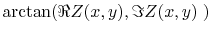
To reduce the time needed for analysis and printing,
I reduced the data size two different ways,
by decimation and local averaging,
as shown in Figure 12.
The decimation was to about 1 part in 9 on each axis,
and the local averaging was done in  windows
giving the same spatial resolution in each case.
The local averaging was done independently in the
plane of the real part and the plane of the imaginary part.
On the smoothed data the phase is less noisy.
windows
giving the same spatial resolution in each case.
The local averaging was done independently in the
plane of the real part and the plane of the imaginary part.
On the smoothed data the phase is less noisy.
|
|---|
squeeze
Figure 12.
Phase based on decimated data (left)
and smoothed data (right).
|
|---|
|
|
|---|
From Figures 11 and 12,
we see that contours of constant phase
appear to be contours of constant altitude;
this conclusion leads us to suppose that a study of radar theory
would lead us to a relation like
 ,
where
,
where  is altitude.
We nonradar specialists often think of phase in
is altitude.
We nonradar specialists often think of phase in
 as being caused by some time delay and
being defined for some constant frequency
as being caused by some time delay and
being defined for some constant frequency  .
Knowledge of this (as well as some angle parameters)
would define the physical units of .
.
Knowledge of this (as well as some angle parameters)
would define the physical units of .
Because the flat land away from the mountain is all at the same phase
(as is the altitude),
the distance as revealed by the phase does not represent
the distance from the ground to the satellite viewer.
We are accustomed to measuring altitude along a vertical line to a datum;
but here, the distance seems to be measured
from the ground along a  angle from the vertical
to a datum at the satellite height.
angle from the vertical
to a datum at the satellite height.
Phase is a troublesome measurement, because
we generally see it modulo  .
Marching up the mountain, we see the phase getting lighter and lighter
until it suddenly jumps to black, which then continues to lighten
as we continue up the mountain to the next jump.
Let us undertake to compute the phase, including
all its jumps of .
Begin with a complex number
.
Marching up the mountain, we see the phase getting lighter and lighter
until it suddenly jumps to black, which then continues to lighten
as we continue up the mountain to the next jump.
Let us undertake to compute the phase, including
all its jumps of .
Begin with a complex number  representing
the complex-valued image at any location
in the
representing
the complex-valued image at any location
in the  -plane.
Computers find the imaginary part of the logarithm
with the arctan function of two arguments, atan2(y,x),
which puts the phase in the range
 ,
although any multiple of could be added.
We seem to escape the
,
although any multiple of could be added.
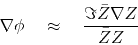
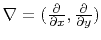
We seem to escape the  phase ambiguity by differentiating:
 |
|
|
(87) |
For every point on the  -axis, equation (87)
is a differential equation on the
-axis, equation (87)
is a differential equation on the  -axis.
We could integrate them all to find
-axis.
We could integrate them all to find  .
That sounds easy.
On the other hand,
the same equations are valid when and are interchanged,
therefore we get twice as many equations as unknowns.
Ideally either of these sets of equations
is equivalent to the other;
but for real data, we expect to be fitting this fitting goal:
.
That sounds easy.
On the other hand,
the same equations are valid when and are interchanged,
therefore we get twice as many equations as unknowns.
Ideally either of these sets of equations
is equivalent to the other;
but for real data, we expect to be fitting this fitting goal:
 |
(88) |
where
 .
Mathematically, computing phase this way
is like our previous seismic flattening with
.
Mathematically, computing phase this way
is like our previous seismic flattening with
 .
Taking measurements to be phase differences
between neighboring mesh points,
it is more correct to interpret Equation (88) as
a difference equation than a differential equation.
Because we measure phase differences only over tiny distances (one pixel),
we hope not to worry about phases greater than .
But, if such jumps do occur, the jumps contribute to overall error.
.
Taking measurements to be phase differences
between neighboring mesh points,
it is more correct to interpret Equation (88) as
a difference equation than a differential equation.
Because we measure phase differences only over tiny distances (one pixel),
we hope not to worry about phases greater than .
But, if such jumps do occur, the jumps contribute to overall error.
Let us consider a typical location in the plane where the complex numbers
 are given. Define a shorthand
  , and
, and  as follows:
![\begin{displaymath}
\left[
\begin{array}{ll}
a & b \\
c & d
\end{array} \r...
... & Z_{i,j+1} \\
Z_{i+1,j} & Z_{i+1,j+1}
\end{array} \right]
\end{displaymath}](img377.png) |
(89) |
With this shorthand, the difference equation representation of the fitting goal (88) is:
 |
(90) |
Now, let us find the phase jumps between the various locations. Complex numbers  and
and  may be expressed in polar form, say
 and
and
 .
The complex number
.
The complex number
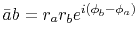 has the desired phase
 .
To obtain it we take the imaginary part of the complex logarithm
.
To obtain it we take the imaginary part of the complex logarithm
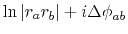 :
:
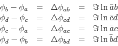 |
(91) |
which gives the information needed to fill in the right side of
(90), as done by subroutine igrad2init() from
module unwrap ![[*]](icons/crossref.png) .
.
The operator needed is igrad2,
gradient with its adjoint, the divergence.
Subsections
|
|
|
|
| Model fitting by least squares | |
|
Next: Estimating the inverse gradient
Up: Model fitting by least
Previous: Gulf of Mexico Salt
2014-12-01