GEO 365N/384S Seismic Data Processing Computational Assignment 3

DMO

In this section, we will apply an improved method of stacking (Fowler, 1988) to the same dataset.

1. Change directory to hw3/dmo.
2. Run

   scons -c
   

   to remove (clean) previously generated files.
3. The method starts with generating an ensemble of NMO stacks with constant velocities (Figure 8.)

   

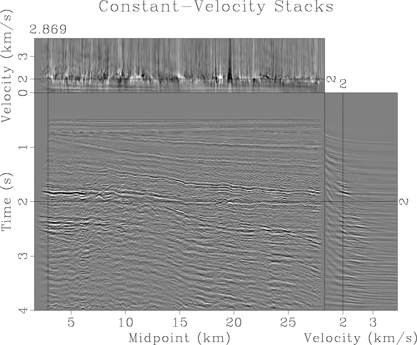
   stacks
   Figure 8. Viking Graben dataset after NMO stacking with an ensemble of constant velocities.

   

   
   

   To generate the stacks and display them on your screen, run

   scons stacks.view
   

4. Fowler's method works by transforming the stack volume into the frequency-wavenumber $\{\omega,k\}$ domain and applying the velocity mapping according to
   

   $$v_0 = \displaystyle v\,\left(1+\frac{k^2\,v^2}{4\,\omega^2}\right)^{-1/2}\;,$$ (1)

   
   
   where $v$ is NMO stacking velocity (dip-dependent) and $v_0$ is time-migration velocity (dip-independent).

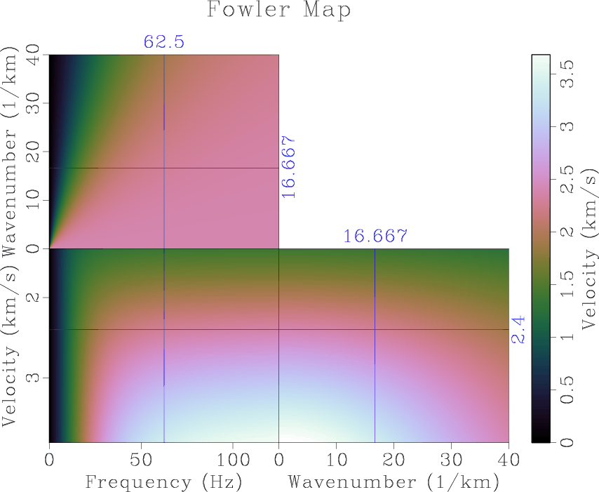
   The map defined by equation (1) is shown in Figure 9. To display it, run

   scons map.view
   

   map Figure 9. Fourier-domain velocity map used in Fowler's DMO method.

5. To perform the DMO correction of the constant-velocity stacks (Figure 10), run

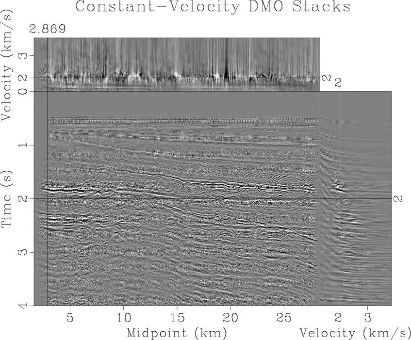
   scons dmo.view
   

   Compare the results by running

   sfpen Fig/dmo.vpl Fig/stacks.vpl
   

   Do you notice any improvements?

   

   

   dmo
   Figure 10. Viking Graben dataset after DMO stacking with an ensemble of constant velocities.

   

   
   

6. Fowler's method does not generate semblance scans, but it is possible to pick velocities using the power of the stack or the envelope.

   To pick the DMO-corrected velocity automatically from the envelope (Figure 11), run

   scons vpick.view
   

   

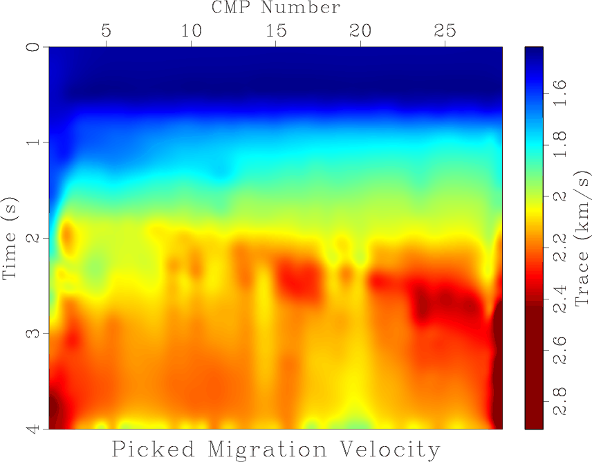
   vpick
   Figure 11. Migration velocity picked automatically from DMO stacks.

   

   
   

7. After the velocity is picked, we can generate a DMO stack by slicing through the velocity cube.

   Run

   scons slice.view
   

   to see the result (Figure 12.)

   

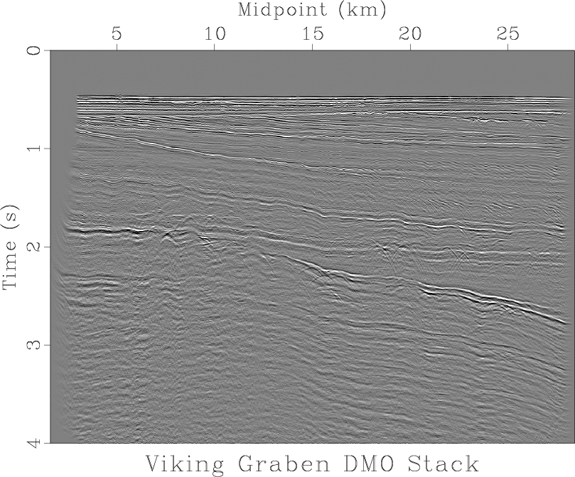
   slice
   Figure 12. DMO stack generated by slicing the constant-velocity stacks.

   

   
   

8. To evaluate the velocity picking and to observe the change brought by DMO, we can examine a particular CMP location. Run

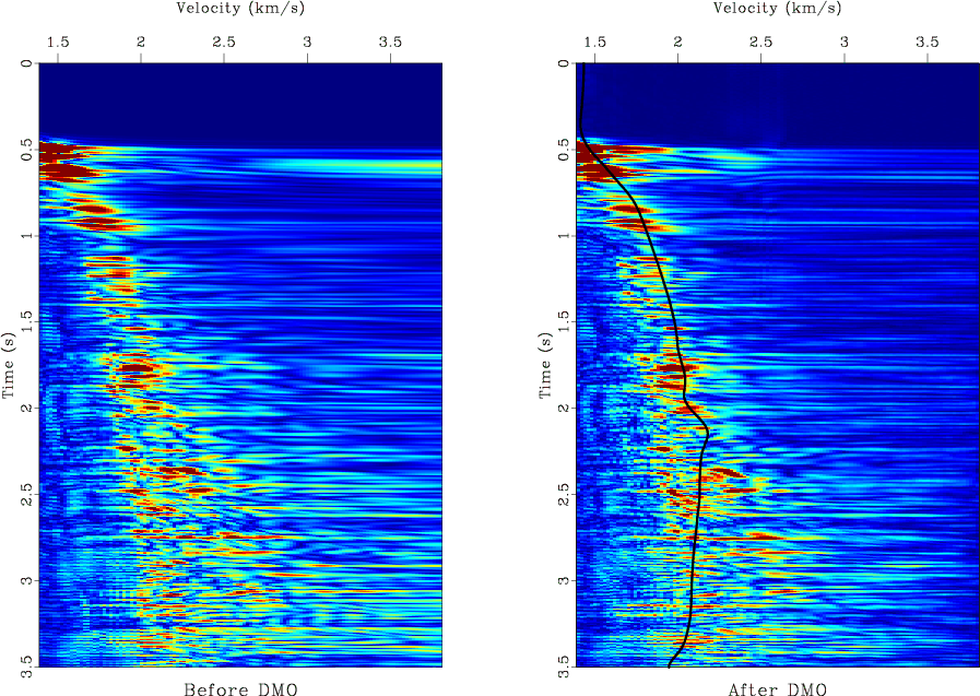
   scons envelope.view
   

   to display the result (Figure 13.)

   Modify the SConstruct file to try several other CMP locations and select one that shows the most interesting change.

   envelope Figure 13. Comparison of velocity analysis before and after DMO at a selected CMP location.

9. Similarly to the previous section, you creative task is to improve the stack (Figure 12) by improving the result of automatic picking. You can use any tools to find a better slice through the velocity cube. Document your work and include the results in this document.

10. For an EXTRA CREDIT, use the materials of Computational Assignment 2 to perform Stolt migration of the DMO stack without leaving the Fourier transform. Note that you can also pick velocities after migration. Does it improve the migration results?

from rsf.proj import *

# Download pre-processed CMP gathers
# from the Viking Graben dataset
Fetch('paracdp.segy','viking')

# Convert to RSF
Flow('paracdp tparacdp','paracdp.segy',
     'segyread tfile=${TARGETS[1]}')

# Convert to CDP gathers, time-power gain and high-pass filter
Flow('cmps','paracdp',
     '''
     intbin xk=cdpt yk=cdp | window max1=4 | 
     pow pow1=2 | bandpass flo=5 |
     put label3=Midpoint unit3=km o3=1.619 d3=0.0125
     ''')

# Extract offsets
Flow('offsets mask','tparacdp',
     '''
     headermath output=offset | 
     intbin head=$SOURCE xk=cdpt yk=cdp mask=${TARGETS[1]} | 
     dd type=float |
     scale dscale=0.001
     ''')

# Window bad traces
Flow('maskbad','cmps',
     'mul $SOURCE | stack axis=1 | mask min=1e-20')

Flow('mask2','maskbad mask','spray axis=1 n=1 | mul ${SOURCES[1]}')

# NMO stack with an ensemble of constant velocities
Flow('stacks','cmps offsets mask2',
     '''
     stacks half=n v0=1.4 nv=121 dv=0.02 
     offset=${SOURCES[1]} mask=${SOURCES[2]}
     ''',split=[3,'omp'])

# Taper midpoint
Flow('stackst','stacks','costaper nw3=100')

Result('stacks','stackst',
       '''
       byte gainpanel=all | transp plane=23 memsize=5000 |
       grey3 frame1=500 frame2=100 frame3=30 point1=0.8 point2=0.8
       title="Constant-Velocity Stacks" label3=Velocity unit3=km/s
       ''')

# Apply double Fourier transform (cosine transform)
Flow('cosft','stackst','pad n3=2401 | cosft sign1=1 sign3=1')

# Transpose f-v-k to v-f-k
Flow('transp','cosft','transp',split=[3,'omp'])

# Fowler DMO: mapping velocities
Flow('map','transp',
     '''
     math output="x1/sqrt(1+0.25*x3*x3*x1*x1/(x2*x2))" | 
     cut n2=1
     ''')

Result('map',
       '''
       byte gainpanel=all allpos=y bar=bar.rsf | 
       grey3 title="Fowler Map" label1=Velocity 
       unit1=km/s label3=Wavenumber barlabel=Velocity barunit=km/s
       frame1=50 frame2=500 frame3=1000 color=x scalebar=y 
       ''')

Flow('fowler','transp map','iwarp warp=${SOURCES[1]} | transp',
     split=[3,'omp'])

# Inverse Fourier transform
Flow('dmo','fowler','cosft sign1=-1 sign3=-1 | window n3=2142')

Result('dmo',
       '''
       byte gainpanel=all | transp plane=23 memsize=5000 |
       grey3 frame1=500 frame2=100 frame3=30 point1=0.8 point2=0.8
       title="Constant-Velocity DMO Stacks" 
       label3=Velocity unit3=km/s
       ''')

# Compute envelope for picking
Flow('envelope','dmo','envelope | scale axis=2',split=[3,'omp'])

# Pick velocity
Flow('vpick','envelope','pick rect1=25 rect2=50 vel0=1.45')

Result('vpick',
       '''
       grey mean=y color=j scalebar=y barreverse=y barunit=km/s
       title="Picked Migration Velocity" label2="CMP Number" unit2= 
       ''')

# Take a slice
Flow('slice','dmo vpick','slice pick=${SOURCES[1]}')

Result('slice','grey title="Viking Graben DMO Stack" ')

# Check one CMP location

p = 1500 # !!! MODIFY ME !!!

Flow('before','stackst','window n3=1 f3=%d | envelope' % p)
Flow('after','envelope','window n3=1 f3=%d' % p)

for case in ('before','after'):
    Plot(case,
         '''
         window max1=3.5 |
         grey color=j allpos=y title="%s DMO" 
         label2=Velocity unit2=km/s
         ''' % case.capitalize())

Flow('vpick1','vpick','window n2=1 f2=%d' % p)
Plot('vpick1',
     '''
     graph yreverse=y transp=y plotcol=7 plotfat=7 
     pad=n min2=1.4 max2=3.8 wantaxis=n wanttitle=n
     ''')
Plot('after2','after vpick1','Overlay')

Result('envelope','before after2','SideBySideAniso')

End()

GEO 365N/384S Seismic Data Processing Computational Assignment 3