|
|
|
|
Multichannel adaptive deconvolution based on streaming prediction-error filter |
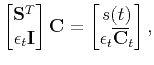
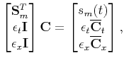
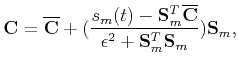
Equation 3 can be written in terms of a shortened block-matrix notation
Assuming that adjacent filter coefficients are similar, the current filter
coefficients at a certain point can be constrained by the adjacent filter
coefficients in both time and space directions, and the regularization
constraint terms are
![]() and
and
![]() .
.
![]() and
and
![]() are weights for regularization constraint
terms along time and space directions, respectively, which control the
similarity of the adjacent filter coefficients. In this case, the
underdetermined problem is transformed into an overdetermined problem.
The filter coefficients are calculated by solving the regularized
autoregression problem
are weights for regularization constraint
terms along time and space directions, respectively, which control the
similarity of the adjacent filter coefficients. In this case, the
underdetermined problem is transformed into an overdetermined problem.
The filter coefficients are calculated by solving the regularized
autoregression problem
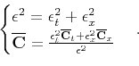
The Sherman-Morrison formula in linear algebra (Hager, 1989) is able to directly transform the inverse matrix in equation 7 without iterations:
Equation 9 shows that the adaptive coefficients get updated by adding a scaled version of the data, and the scale is proportional to the streaming prediction error. Updating the filter coefficients requires only elementary algebraic operation without iteration.
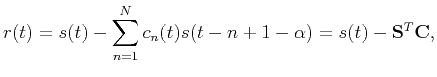
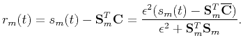
According to the definition of prediction error (equation 1) and prediction coefficients (equation 9), the deconvolution result of streaming PEF can be expressed as
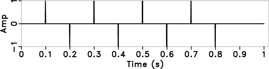
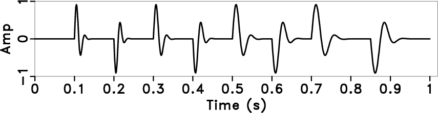
In this paper, we select the minimum-phase wavelet as the source wavelet to verify the effectiveness of the proposed deconvolution method. The minimum-phase wavelet can be expressed as
The minimum-phase wavelet (figure 1a) and the
sequence of reflection coefficients (figure 1b)
generate a simple 1D convolution model (figure 1c)
, where the wavelet frequencies corresponding to every two reflection
coefficients with opposite amplitude are selected to be 45 Hz, 35 Hz, 25 Hz,
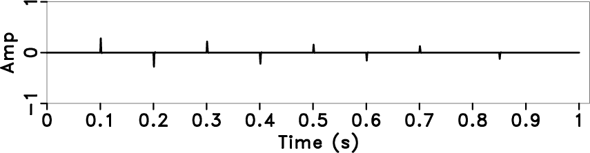
and 20 Hz, respectively. Figure 1d is the result
by using the streaming PEF deconvolution (![]() ,
,
![]() , and
, and
![]() ). The streaming PEF deconvolution method effectively improve the
time resolution, however, the relative amplitude relationship among
different reflections has been changed, which occur more in predictive
deconvolution methods. Notice that the amplitude distortion is related to
the dominant frequency of the wavelet: the lower dominant frequency is,
the worse amplitude fidelity is shown because the peak amplitude of
minimum-phase wavelets is hard to happen in the first sample point.
). The streaming PEF deconvolution method effectively improve the
time resolution, however, the relative amplitude relationship among
different reflections has been changed, which occur more in predictive
deconvolution methods. Notice that the amplitude distortion is related to
the dominant frequency of the wavelet: the lower dominant frequency is,
the worse amplitude fidelity is shown because the peak amplitude of
minimum-phase wavelets is hard to happen in the first sample point.

|
|---|
|
wave,refl,in,spef1
Figure 1. Analysis of amplitude distortion for streaming PEFs. Minimum-phase wavelet (a), the reflectivity (b), the nonstationary synthetic seismic trace (c), and the deconvolution result by using streaming PEF with constant prediction step (d). |
|
|
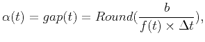
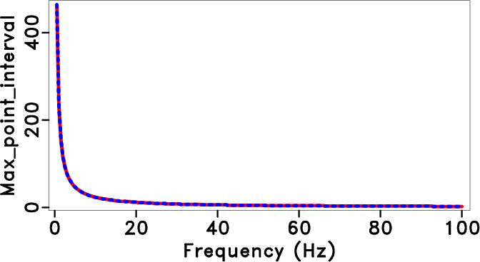
The red line in figure 2 represents the theoretical curve of sample number between the start point and peak-amplitude point of minimum-phase wavelets, which is the function of the dominant frequency. We select an empirical equation to fit the curve as follows:
|
|---|
|
gapdif
Figure 2. Parameter |
|
|
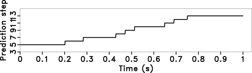
Figure 3a shows the local frequency calculated from
the synthetic trace (figure 1c), and the
time-varying prediction steps (figure 3b) are obtained
according to equation 14, where the parameter ![]() is 0.232 and the
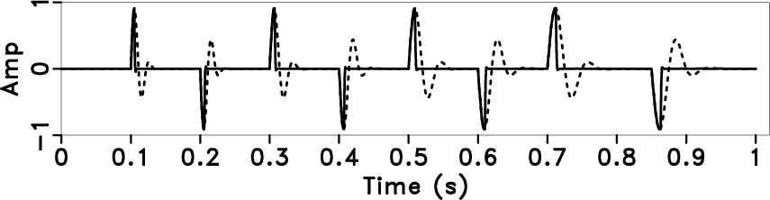
time interval is 1 ms. Figure 3c shows the result
processed by the streaming PEF deconvolution with the time-varying
predictionstep. Compared with original data (dotted line in
figure 3c), the proposed method keeps the relative
amplitude relationship in the deconvolution result
(solid line in figure 3c) at the cost of a lower
resolution improvement.
is 0.232 and the
time interval is 1 ms. Figure 3c shows the result
processed by the streaming PEF deconvolution with the time-varying
predictionstep. Compared with original data (dotted line in
figure 3c), the proposed method keeps the relative
amplitude relationship in the deconvolution result
(solid line in figure 3c) at the cost of a lower
resolution improvement.

|
|---|
|
lfe,vvlag,dif
Figure 3. The deconvolution result by using the streaming PEF with time-varying prediction steps. The local frequency (a), time-varying prediction step (b), the deconvolution result with the proposed method (solid line), which is compared with the original trace (dotted line) (c). |
|
|
The proposed method mainly includes four parameters: the filter length
(![]() ), time constraint factor (
), time constraint factor (
![]() ), spatial constraint factor
(
), spatial constraint factor
(
![]() ) and constant
) and constant ![]() . According to the experiment, a reasonable
deconvolution results can be obtained when
. According to the experiment, a reasonable
deconvolution results can be obtained when ![]() . The constraint factors
. The constraint factors
![]() and
and
![]() are the key parameters for the proposed method.
The denominator in equation 9 suggests that
are the key parameters for the proposed method.
The denominator in equation 9 suggests that
![]() and
and
![]() should have the same order of the magnitude as
should have the same order of the magnitude as
![]() . Too small a constraint factor would make the
deconvolution results unstable, and too large a constraint factor would lead
to the filter coefficients not being updated effectively. When the filter
coefficients are constrained only in the time direction, it is only necessary
to set the spatial constraint factor to zero (
. Too small a constraint factor would make the
deconvolution results unstable, and too large a constraint factor would lead
to the filter coefficients not being updated effectively. When the filter
coefficients are constrained only in the time direction, it is only necessary
to set the spatial constraint factor to zero (
![]() ). In theory,
the
). In theory,
the ![]() value is the ratio of the peak-amplitude time to the period
of the wavelet. For minimum-phase wavelets,
value is the ratio of the peak-amplitude time to the period
of the wavelet. For minimum-phase wavelets, ![]() is typically less than 0.25.
is typically less than 0.25.
Like the traditional predictive deconvolution, the relative amplitude relationship of the results that are generated by streaming PEF deconvolution with constant prediction step is not consistent with the original data, so we introduce the time-varying prediction step and derive its empirical formula. After adding the time-varying prediction step, the amplitude of the deconvolution result of the synthetic model (figure 3) tends to be consistent with the true amplitude of the original data. However, the actual seismic data is complex due to the earth absorption attenuation and other factors, so the amplitude of deconvolution results is not true amplitude, but its relative amplitude relationship is closer to the original data.
Since the proposed method can adaptively update the filter coefficients without iteration and characterize the nonstationary properties of the data, both the storage and computational cost of the filters are less than those of the adaptive predictive filtering methods based on the iterative algorithms. Table 1 compares the storage and computational cost of the different methods.
The proposed filter is constrained in both the time and space directions while the filter is still one-dimensional, that is, the multichannel adaptive deconvolution technology is based on the streaming PEF with one-dimensional structure and two-dimensional constraints. To ensure the stability of the calculation, the first boundary trace only uses the time constraint condition to compute the streaming PEF coefficients, and the constraints in both space and time directions are added to the other trace. An extension of the proposed method to 3D is straightforward and provides a fast adaptive multichannel deconvolution implementation for high-dimensional seismic data.
| Method | Storage | Cost |
| Stationary PEF |
|
|
| 1D nonstationary PEF with iterative algorithm |
|
|
| 1D streaming PEF | ||
| 2D streaming PEF |
|
|
|
|
|
Multichannel adaptive deconvolution based on streaming prediction-error filter |