|
|
|
|
Adaptive prediction filtering in |
Equation 5 shows that one sample in ![]() -
-![]() domain can be
predicted by the samples in adjacent traces with weight coefficients
domain can be
predicted by the samples in adjacent traces with weight coefficients
![]() , which is time- and space-varying. The equation assumes
that the seismic data only consist of plane waves
, which is time- and space-varying. The equation assumes
that the seismic data only consist of plane waves
![]() and random noise
that corresponds to a least-squares error.
and random noise
that corresponds to a least-squares error.
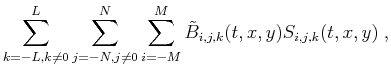
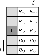
Figure 1a shows a 2D space-causal APF
structure, which is time-noncausal filter. White grids stand for
prediction samples and the dark-grey grid is the output (or target)
position, while light-grey grids are unused samples. The filter size
of the space-causal APF is
![]() . Meanwhile, space-noncausal
APF (Figure 1b) has a symmetric structure
along time and space axes. The filter size of the space-noncausal APF
is
. Meanwhile, space-noncausal
APF (Figure 1b) has a symmetric structure
along time and space axes. The filter size of the space-noncausal APF
is
![]() . The 3D
. The 3D ![]() -
-![]() -
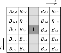
-![]() APF also has space-causal or
space-noncausal structure, Figure 2 shows the
noncausal one. In a 3D seismic datacube, the plane events can be
predicted along two different spatial directions. A 2D
APF also has space-causal or
space-noncausal structure, Figure 2 shows the
noncausal one. In a 3D seismic datacube, the plane events can be
predicted along two different spatial directions. A 2D ![]() -
-![]() APF
will have difficulty preserving accurate plane waves because it only
uses the information in
APF
will have difficulty preserving accurate plane waves because it only
uses the information in ![]() or
or ![]() direction, however, a 3D
direction, however, a 3D
![]() -
-![]() -
-![]() APF provides a more natural structure.
APF provides a more natural structure. ![]() -
-![]() -
-![]() adaptive prediction filtering for random noise attenuation follows two
steps:
adaptive prediction filtering for random noise attenuation follows two
steps:
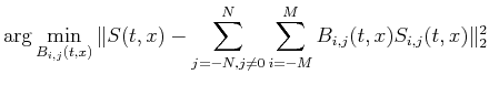
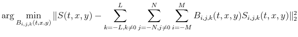
1. Estimating 3D space-noncausal APF coefficients
![]() by solving the regularized least-squares
problem (equation 4 or 5 in 2D):
2pt
by solving the regularized least-squares
problem (equation 4 or 5 in 2D):
2pt
2. Calculating noise-free signal
![]() according to
2pt
according to
2pt
|
|---|
|
causal2d,noncausal2d
Figure 1. Schematic illustration of a 2D |
|
|
|
|---|
|
noncausal3d
Figure 2. Schematic illustration of a 3D |
|
|
|
|
|
|
Adaptive prediction filtering in |
![$\displaystyle + \epsilon^2 \sum_{j=-N,j\neq0}^{N} \sum_{i=-M}^{M}
\Vert\mathbf{R}[B_{i,j}(t,x)]\Vert _2^2\;,$](img26.png)
![$\displaystyle + \epsilon^2 \sum_{k=-L,k\neq0}^{L} \sum_{j=-N,j\neq0}^{N}
\sum_{i=-M}^{M}
\Vert\mathbf{R}[B_{i,j,k}(t,x,y)]\Vert _2^2\;,$](img33.png)