|
|
|
|
Adaptive prediction filtering in |
Another approach is to apply nonstationary filters. The denoised
results by using ![]() -
-![]() RNA and
RNA and ![]() -
-![]() APF are shown in
Figure 5a and
5c, respectively. The filter length
of
APF are shown in
Figure 5a and
5c, respectively. The filter length
of ![]() -
-![]() RNA is 8 and it has a 10-sample (frequency) and 20-sample
(space) smoothing radius.
RNA is 8 and it has a 10-sample (frequency) and 20-sample
(space) smoothing radius. ![]() -
-![]() RNA
(Figure 5a) has a better result
than stationary methods, e.g.,
RNA
(Figure 5a) has a better result
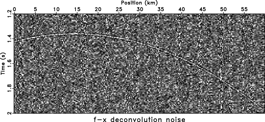
than stationary methods, e.g., ![]() -
-![]() deconvolution
(Figure 4a) and
deconvolution
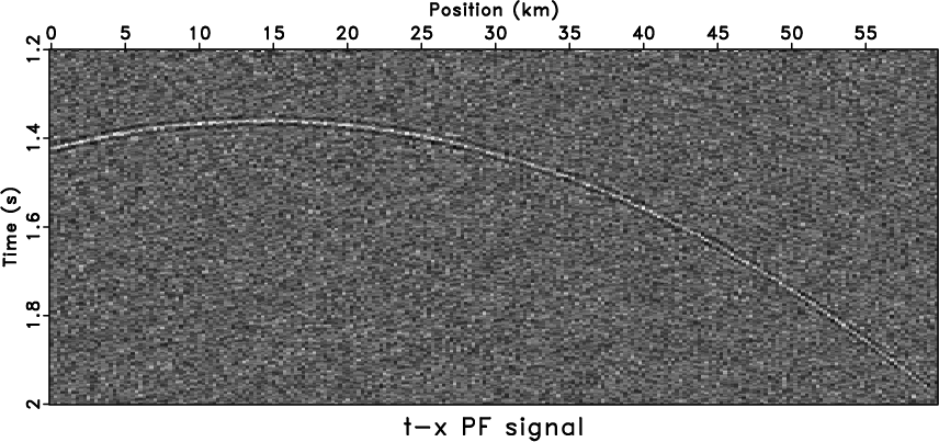
(Figure 4a) and ![]() -
-![]() PF
(Figure 4c), however, there is
still signal trend in the noise section
(Figure 4b) and artificial
events appear that are similar to those from
PF
(Figure 4c), however, there is
still signal trend in the noise section
(Figure 4b) and artificial
events appear that are similar to those from ![]() -
-![]() deconvolution. For the
deconvolution. For the ![]() -
-![]() APF, the choice of the filter length in
space is similar to that in
APF, the choice of the filter length in
space is similar to that in ![]() -
-![]() RNA. We tend to use a 12-sample
filter in space, and the filter length in time for the
RNA. We tend to use a 12-sample
filter in space, and the filter length in time for the ![]() -
-![]() APF is
selected to five samples. As the time-length of the
APF is
selected to five samples. As the time-length of the ![]() -
-![]() APF
increases, the
APF
increases, the ![]() -
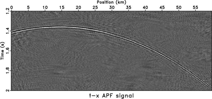
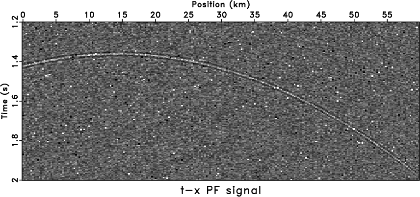
-![]() APF passes more random noise. We use the
shaping regularization with a 60-sample (time) and 20-sample (space)
smoothing radius to constrain the APF coefficient space. The denoised
result and removed noise are shown in
Figure 5c and
5d, respectively.
APF passes more random noise. We use the
shaping regularization with a 60-sample (time) and 20-sample (space)
smoothing radius to constrain the APF coefficient space. The denoised
result and removed noise are shown in
Figure 5c and
5d, respectively. ![]() -
-![]() APF also
introduces a few artifacts, but the artifacts show a random-trend
distribution
(Figure 5c). Meanwhile, the
APF also
introduces a few artifacts, but the artifacts show a random-trend
distribution
(Figure 5c). Meanwhile, the ![]() -
-![]() APF, shown in Figure 5d, preserves
signal better than the
APF, shown in Figure 5d, preserves
signal better than the ![]() -
-![]() RNA.
RNA.
|
|---|
|
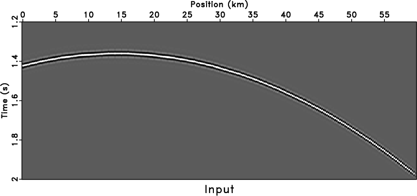
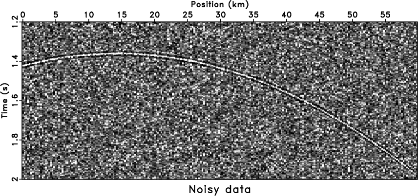
jcacov,noiz
Figure 3. Curved model (a) and noisy data (b). |
|
|


|
|---|
|
fxpatch,fxdiff,txpatch,txdiff
Figure 4. Comparison of stationary methods. The denoised result by |
|
|


|
|---|
|
fxrna,fxnoiz,aspred,asnoiz
Figure 5. Comparison of nonstationary methods. The denoised result by |
|
|
For further discussion, we added extra spike noise to
Figure 3b, the new noisy model with a wiggle display
is shown in Figure 6a. When
comparing with the ![]() -
-![]() PF with patching
(Figure 6b) and the
PF with patching
(Figure 6b) and the ![]() -
-![]() RNA
(Figure 6c), the
RNA
(Figure 6c), the ![]() -
-![]() APF
shows better signal-protection ability, however, the quality of the
denoised result gets worse than
Figure 5c because of the spikes
(Figure 6d). Larger smoothing
radius can reduce the artifacts at the cost of attenuating part of the
signals.
APF
shows better signal-protection ability, however, the quality of the
denoised result gets worse than
Figure 5c because of the spikes
(Figure 6d). Larger smoothing
radius can reduce the artifacts at the cost of attenuating part of the
signals.


|
|---|
|
noiz1,txpatch1,fxrna1,aspred1
Figure 6. Tests of hybrid noise model by using different methods. Data with hybrid noise (a), |
|
|
|
|
|
|
Adaptive prediction filtering in |