|
|
|
|
Adaptive prediction filtering in |
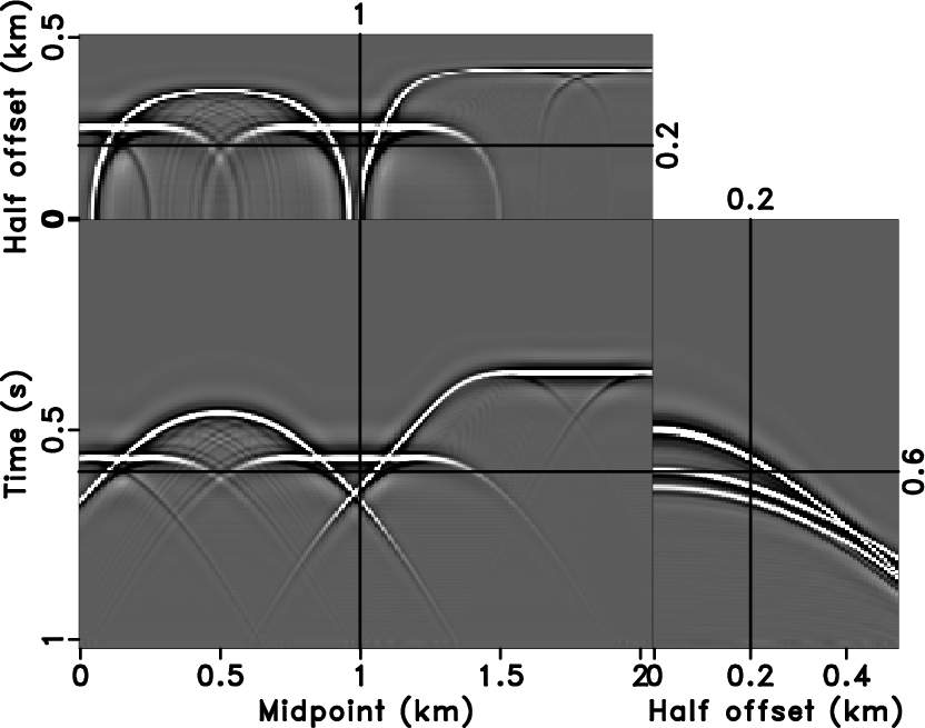
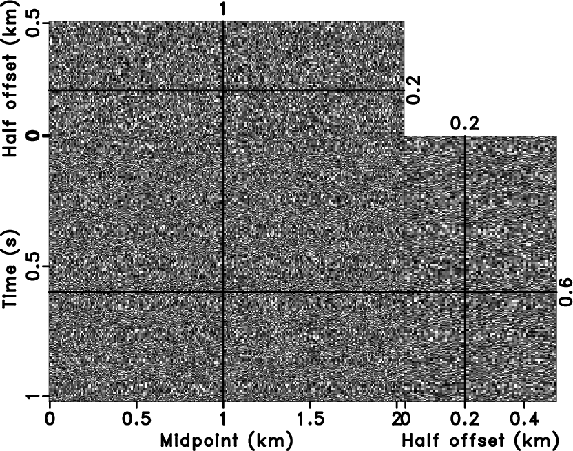
We created a 3D example by Kirchhoff modeling
(Figure 9a), the corresponding velocity model is
a slice out of the benchmark French model
(Liu and Fomel, 2010; French, 1974). Three surfaces of
Figure 9a illustrate the corresponding slices at
time=0.6s, midpoint=1.0km, and
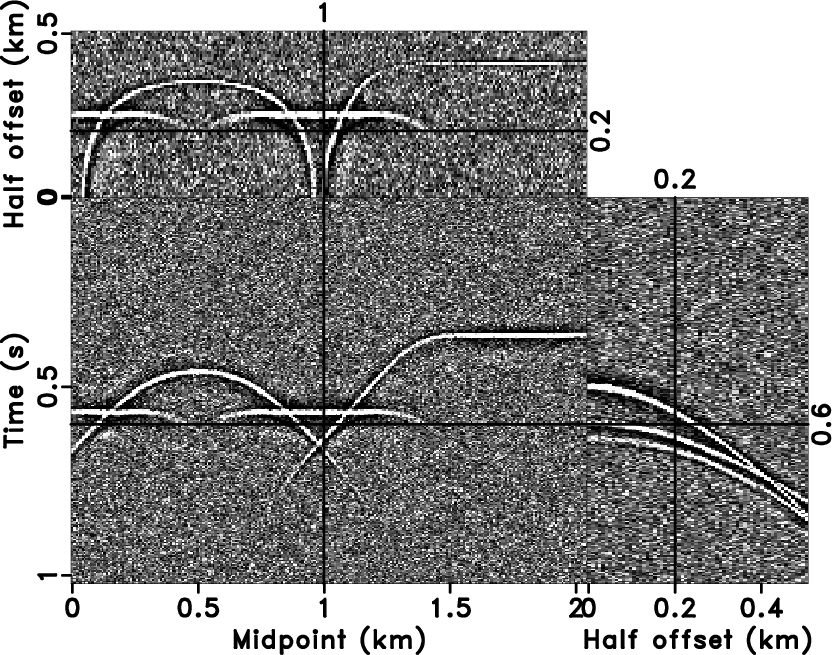
half-offset=0.2km. Figure 9b is the noisy
data. The challenge in this example is to account for multi-dimension,
nonstationarity, and conflicting dips. For comparison, we use 3D
![]() -
-![]() -
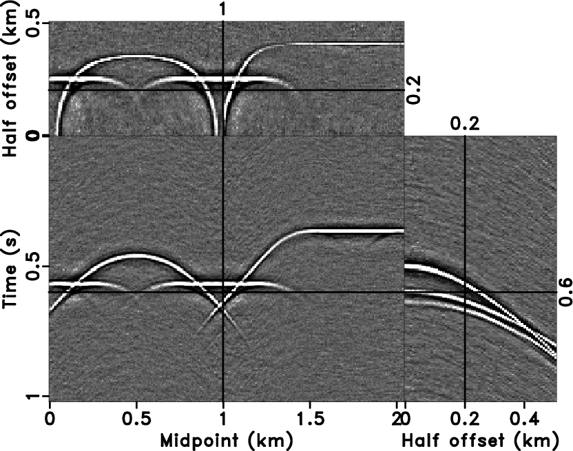
-![]() NRNA (Liu and Chen, 2013) to attenuate random noise
(Figure 10a). The 3D NRNA method
produces a reasonable result. In
Figure 10b, 3D
NRNA (Liu and Chen, 2013) to attenuate random noise
(Figure 10a). The 3D NRNA method
produces a reasonable result. In
Figure 10b, 3D ![]() -
-![]() -
-![]() NRNA shows
a better ability of signal preservation than 2D version
(Liu et al., 2012). However, 3D NRNA still produces artificial events parallel
with curved events. We design a 3D
NRNA shows
a better ability of signal preservation than 2D version
(Liu et al., 2012). However, 3D NRNA still produces artificial events parallel
with curved events. We design a 3D ![]() -
-![]() -
-![]() APF with 5 (time)
APF with 5 (time)
![]() 4 (midpoint)
4 (midpoint) ![]() 4 (half offset) coefficients for each
sample and 15-sample (time), 10-sample (midpoint), and 10-sample (half
offset) smoothing radius to further handle the variability of
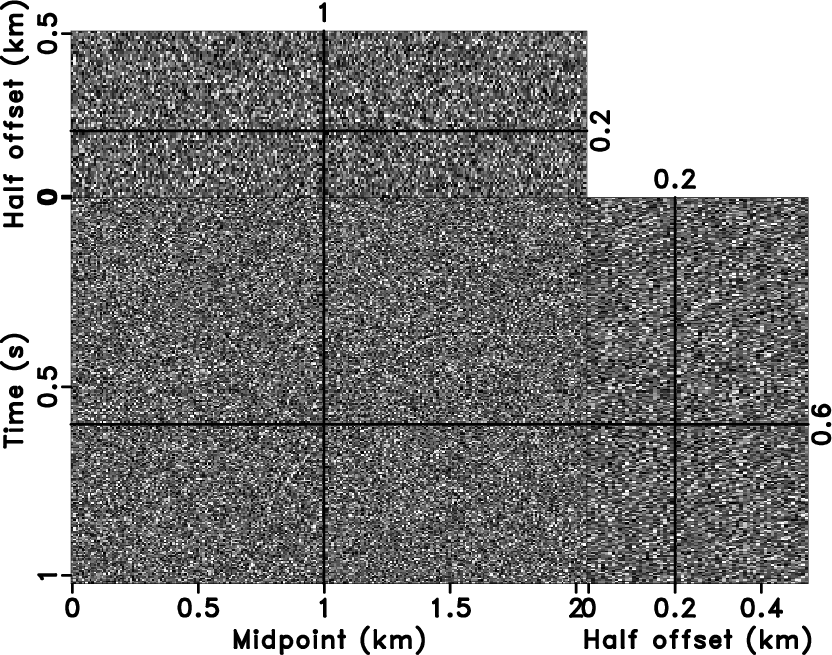
event. Figure 10c and
10d show the denoised result and the
difference between noisy data (Figure 9b) and the
denoised result (Figure 10c) plotted
at the same clip value, respectively. The proposed method succeeds in
the sense that it is hard to distinguish the curved and conflicting
events in the removed noise. Meanwhile, the 3D
4 (half offset) coefficients for each
sample and 15-sample (time), 10-sample (midpoint), and 10-sample (half
offset) smoothing radius to further handle the variability of
event. Figure 10c and
10d show the denoised result and the
difference between noisy data (Figure 9b) and the
denoised result (Figure 10c) plotted
at the same clip value, respectively. The proposed method succeeds in
the sense that it is hard to distinguish the curved and conflicting
events in the removed noise. Meanwhile, the 3D ![]() -
-![]() -
-![]() APF has
fewer artificial events, which are more visible for 3D
APF has
fewer artificial events, which are more visible for 3D ![]() -
-![]() -
-![]() NRNA (Figure 10a).
NRNA (Figure 10a).
|
|---|
|
fdata,fnoise
Figure 9. 3D synthetic data (a) and the corresponding noisy data (b). |
|
|

|
|---|
|
tpre,diff3d,fpred3,ferr3
Figure 10. The denoised result by 3D |
|
|
|
|
|
|
Adaptive prediction filtering in |