|
|
|
|
Inverse B-spline interpolation |
Let us denote the continuous regularization operator by ![]() .
Regularization implies seeking a function
.
Regularization implies seeking a function ![]() such that the
least-squares norm of
such that the
least-squares norm of
![]() is minimum. Using the usual
expression for the least-squares norm of continuous functions and
substituting the basis decomposition (8), we obtain
the expression
is minimum. Using the usual
expression for the least-squares norm of continuous functions and
substituting the basis decomposition (8), we obtain
the expression
We have found a constructive way of creating B-spline regularization operators from continuous differential equations.
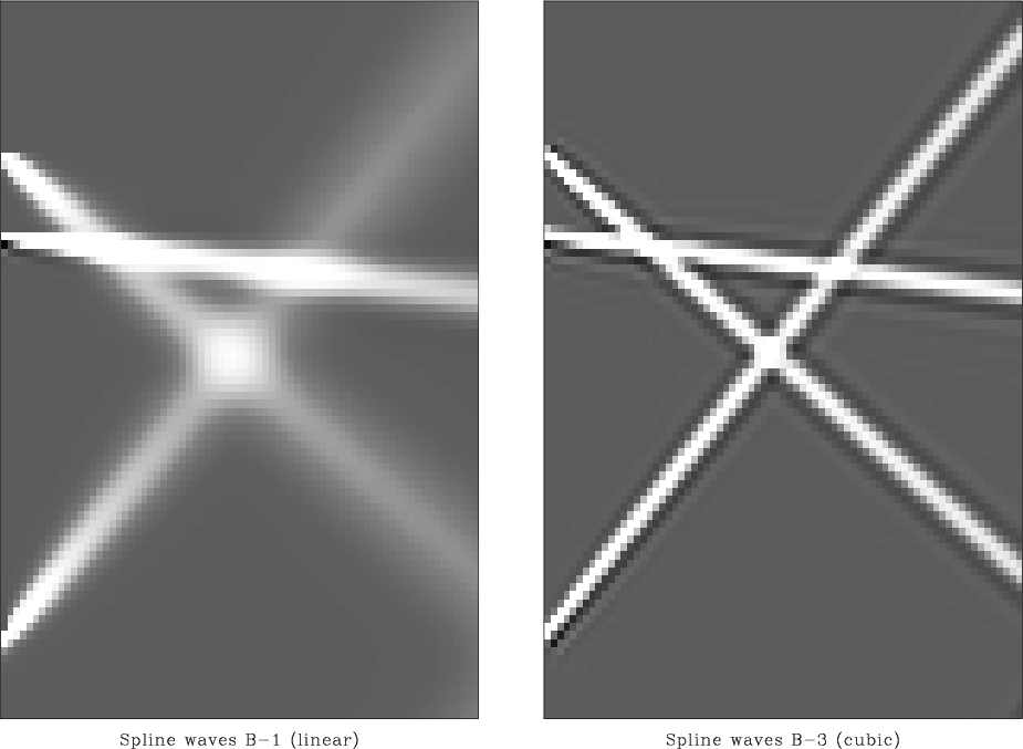
A simple regularization example is shown in Figure 28.
The continuous operator ![]() in this case comes from the theoretical
plane-wave differential equation. I constructed the auto-correlation
filter
in this case comes from the theoretical
plane-wave differential equation. I constructed the auto-correlation
filter ![]() according to formula (24) and factorized it
with the efficient Wilson-Burg method on a helix
(Sava et al., 1998). The figure shows three plane waves
constructed from three distant spikes by applying an inverse recursive
filtering with two different plane-wave regularizers. The left plot
corresponds to using first-order B-splines (equivalent to linear
interpolation). This type of regularizer is identical to Clapp's
steering filters (Clapp et al., 1997) and suffers from numerical
dispersion effects. The right plot was obtained with third-order
splines. Most of the dispersion is suppressed by using a more accurate
interpolation.
according to formula (24) and factorized it
with the efficient Wilson-Burg method on a helix
(Sava et al., 1998). The figure shows three plane waves
constructed from three distant spikes by applying an inverse recursive
filtering with two different plane-wave regularizers. The left plot
corresponds to using first-order B-splines (equivalent to linear
interpolation). This type of regularizer is identical to Clapp's
steering filters (Clapp et al., 1997) and suffers from numerical
dispersion effects. The right plot was obtained with third-order
splines. Most of the dispersion is suppressed by using a more accurate
interpolation.
|
|---|
|
sthree
Figure 28. B-spline regularization. Three plane waves constructed by 2-D recursive filtering with the B-spline plane-wave regularizer. Left: using first-order B-splines (linear interpolation). Right: using third-order B-splines. |
|
|
|
|
|
|
Inverse B-spline interpolation |
![\begin{displaymath}
\left\Vert D\left[f(x)\right]\right\Vert =
\int \left(D...
...(\sum_{k \in K} c_k D\left[ \beta (x-k)\right]\right)^2\,dx\;.
\end{displaymath}](img62.png)
![\begin{displaymath}
\sum_{k \in K} c_k \int D \left[\beta (x-k)\right]
D\left[\beta (x-j)\right] \,dx =
\sum_{k \in K} c_k d_{j-k} = 0\;,
\end{displaymath}](img63.png)
