Forward interpolation

Interpolation theory

Mathematical interpolation theory considers a function $f$, defined on a regular grid $N$. The problem is to find $f$ in a continuum that includes $N$. I am not defining the dimensionality of $N$ and $f$ here because it is not essential for the derivations. Furthermore, I am not specifying the exact meaning of ``regular grid,'' since it will become clear from the analysis that follows. The function $f$ is assumed to belong to a Hilbert space with a defined dot product.

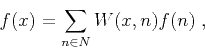
If we restrict our consideration to a linear case, the desired solution will take the following general form

$$f (x) = \sum_{n \in N} W (x, n) f (n)\;,$$ (1)

where $x$ is a point from the continuum, and $W (x, n)$ is a linear weight function that can take both positive and negative values. If the grid $N$ itself is considered as continuous, the sum in formula (1) transforms to an integral in $dn$. Two general properties of the linear weighting function $W (x, n)$ are evident from formula (1).

Property 1  

$$W (n, n) = 1\;.$$ (2)

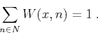
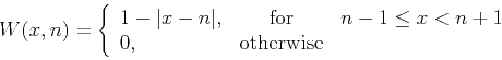
Equality (2) is necessary to assure that the interpolation of a single spike at some point $n$ does not change the value $f (n)$ at the spike.

Property 2  

$$\sum_{n \in N} W (x, n) = 1\;.$$ (3)

This property is the normalization condition. Formula (3) assures that interpolation of a constant function $f (n)$ remains constant.

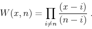
One classic example of the interpolation weight $W (x, n)$ is the Lagrange polynomial, which has the form

$$W (x, n) = \prod_{i \neq n} \frac{(x-i)}{(n-i)}\;.$$ (4)

The Lagrange interpolation provides a unique polynomial, which goes exactly through the data points $f (n)$. The local 1-point Lagrange interpolation is equivalent to the nearest-neighbor interpolation, defined by the formula

$$W (x, n) = \left\{\begin{array}{lcr} 1, & \mbox{for} & n - ... ...leq x < n + 1/2 \\ 0, & \mbox{otherwise} & \end{array}\right.$$ (5)

Likewise, the local 2-point Lagrange interpolation is equivalent to the linear interpolation, defined by the formula

$$W (x, n) = \left\{\begin{array}{lcr} 1 - \vert x-n\vert, & ... ... \leq x < n + 1 \\ 0, & \mbox{otherwise} & \end{array}\right.$$ (6)

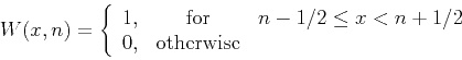
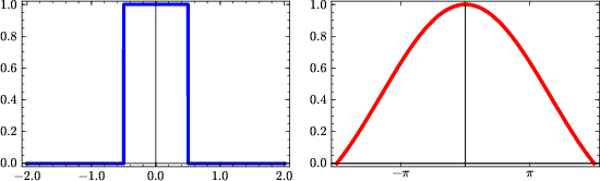
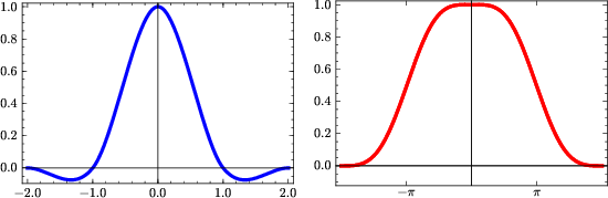
Because of their simplicity, the nearest-neighbor and linear interpolation methods are very practical and easy to apply. Their accuracy is, however, limited and may be inadequate for interpolating high-frequency signals. The shapes of interpolants (5) and (6) and their spectra are plotted in Figures 1 and 2. The spectral plots show that both interpolants act as low-pass filters, preventing the high-frequency energy from being correctly interpolated.

nnint
Figure 1. Nearest-neighbor interpolant (left) and its spectrum (right).

linint
Figure 2. Linear interpolant (left) and its spectrum (right).

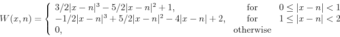
The Lagrange interpolants of higher order correspond to more complicated polynomials. Another popular practical approach is cubic convolution (Keys, 1981). The cubic convolution interpolant is a local piece-wise cubic function:

$$W (x, n) = \left\{\begin{array}{lcr} 3/2 \vert x-n\vert^3 -... ...rt x-n\vert < 2 \\ 0, & \mbox{otherwise} & \end{array}\right.$$ (7)

The shapes of interpolant (7) and its spectrum are plotted in Figure 3.

ccint
Figure 3. Cubic-convolution interpolant (left) and its spectrum (right).

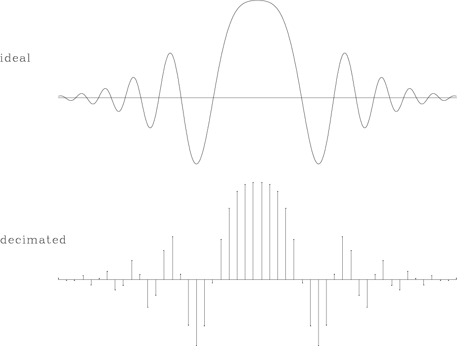
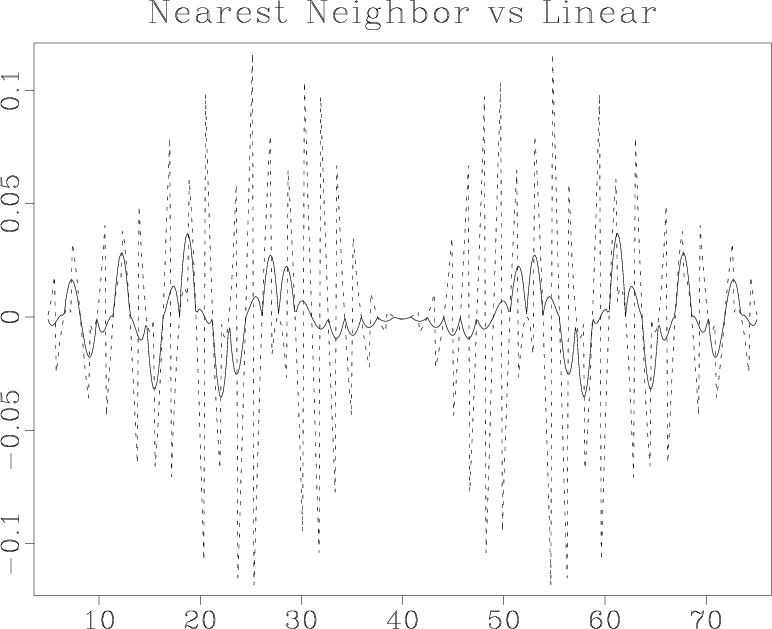
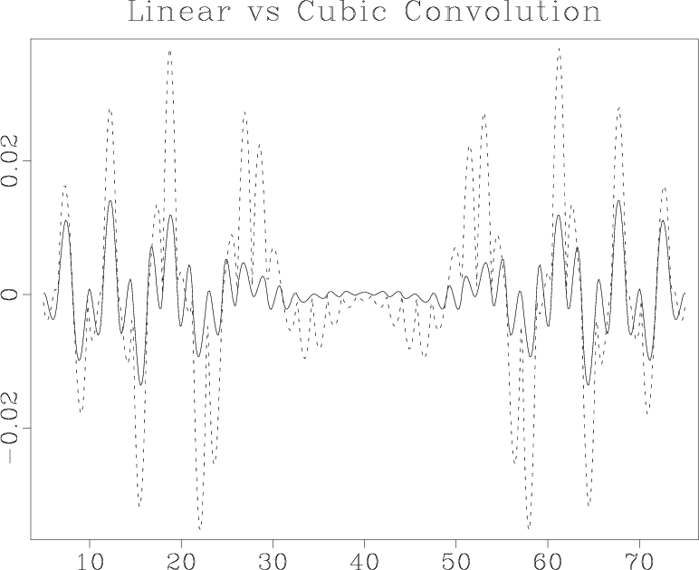
I compare the accuracy of different forward interpolation methods on a one-dimensional signal shown in Figure 4. The ideal signal has an exponential amplitude decay and a quadratic frequency increase from the center towards the edges. It is sampled at a regular 50-point grid and interpolated to 500 regularly sampled locations. The interpolation result is compared with the ideal one. Figures 5 and 6 show the interpolation error steadily decreasing as we proceed from 1-point nearest-neighbor to 2-point linear and 4-point cubic-convolution interpolation. At the same time, the cost of interpolation grows proportionally to the interpolant length.

chirp Figure 4. One-dimensional test signal. Top: ideal. Bottom: sampled at 50 regularly spaced points. The bottom plot is the input in a forward interpolation test.

binlin Figure 5. Interpolation error of the nearest-neighbor interpolant (dashed line) compared to that of the linear interpolant (solid line).

lincub Figure 6. Interpolation error of the linear interpolant (dashed line) compared to that of the cubic convolution interpolant (solid line).

Forward interpolation