|
|
|
|
Multiple realizations using standard inversion techniques |
The missing data problem is probably the simplest to understand and
interpret results.
We begin by binning our data onto a regular mesh.
For ![]() in fitting goals (2) we will use a selector
matrix
in fitting goals (2) we will use a selector
matrix ![]() ,
which is `1' at locations where we have data and `0' at unknown locations.
As an example, let's try to interpolate
a day's worth of data
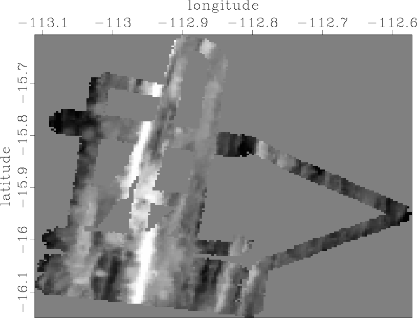
collected by SeaBeam (Figure 1), which measures
water depth under and to the side of a ship (Claerbout, 1998).
,
which is `1' at locations where we have data and `0' at unknown locations.
As an example, let's try to interpolate
a day's worth of data
collected by SeaBeam (Figure 1), which measures
water depth under and to the side of a ship (Claerbout, 1998).
|
init
Figure 1. Depth of the ocean under ship tracks. |
|
|---|---|
|
|
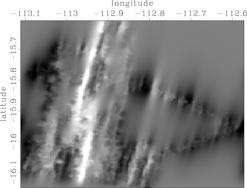
Figure 2 shows the result of estimating a PEF from the known data locations and then using it to interpolate the entire mesh. Note how the solution has a lower spatial frequency as we move away from the recorded data. In addition, the original tracks of the ship are still clearly visible.
|
pef
Figure 2. Result of using a PEF to interpolate Figure 1, taken from GEE. |
|
|---|---|
|
|
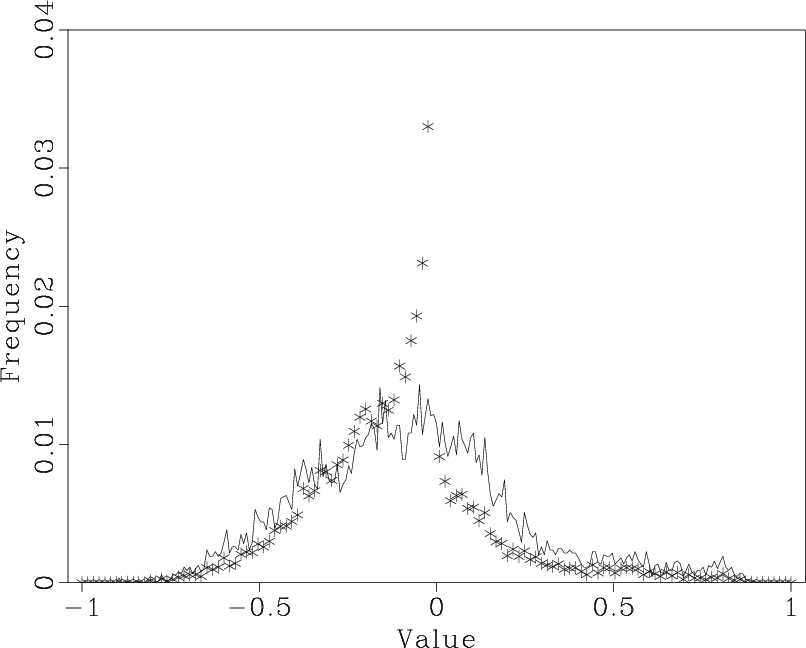
If we look at a histograms of the known data and our estimated data we can see the effect of the PEF. The histogram of the known data has a nice Gaussian shape. The predicted data is much less Gaussian with a much lower variance. We want estimated data to have the same statistical properties as the known data (for a Gaussian distribution this means matching the mean and variance).
|
histo
Figure 3. Histogram for the known data (solid lines) and the estimated data (`*'). Note the dissimilar shapes. |
|
|---|---|
|
|
Geostatisticians are confronted with the same problem. They can produce
smooth, low frequency models through kriging, but must add a little
twist to get model with the statistical properties as the data.
To understand how, a brief review of kriging is necessary.
Kriging estimates each model point by a linear combination of nearby data
points. For simplicity lets assume that the data has a standard
normal distribution.
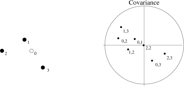
The geostatistician find all of the points ![]() around the point they
are trying to estimate
around the point they
are trying to estimate ![]() . The vector distance between all data points
. The vector distance between all data points
![]() and each data point and the estimation point
and each data point and the estimation point
![]() are then computed.
Using the predefined covariance function estimate
are then computed.
Using the predefined covariance function estimate ![]() , a covariance
value is then extracted
between all known point pairs
, a covariance
value is then extracted
between all known point pairs ![]() and
between known points and
estimation point
and
between known points and
estimation point ![]() at the given distances
at the given distances
![]() and
and
![]() (Figure 4).
They compute the weights (
(Figure 4).
They compute the weights (![]() ) by solving the set
of equations implied by
) by solving the set
of equations implied by
 |
(4) |
|
|---|
|
covar-def
Figure 4. Definition of the terms in equation (3). A vector is drawn between two points. The covariance at the angle and distance describing the vector is then selected. |
|
|
The smooth models provided by kriging often prove
to be poor representations of earth properties.
A classic example is fluid flow where kriged models tend to give inaccurate
predictions. The geostatistical solution
is to perform Gaussian stochastic simulation, rather than kriging, to
estimate the field (Deutsch and Journel, 1992).
There are two major differences between kriging and simulation.
The primary difference
is that a random component is introduced into the estimation process.
Stochastic simulation, or sequential Gaussian simulation, begins
with a random point being selected in the model space.
They then perform kriging, obtaining
a kriged value ![]() and a kriging variance
and a kriging variance ![]() .
Instead of using
.
Instead of using ![]() for the model value we
select a random number
for the model value we
select a random number ![]() from a normal distribution.
We use as our model point estimate
from a normal distribution.
We use as our model point estimate ![]() ,
,
| (5) |
The difference between kriging and simulation has a corollary in our
least squares estimation problem. To see how let's write
our fitting goals in a slightly different format,
By adjusting ![]() we can change the distribution of
we can change the distribution of
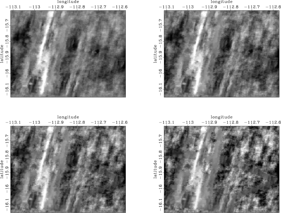
![]() . For example, let's return to the SeaBeam example.
Figure 5 shows four different model estimations
using a normal distribution and various values for the variance.
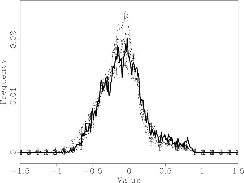
Note how the texture of the model changes significantly. If we look
at a histogram of the various realizations (Figure 6),
we see that the correct
distribution is somewhere between our second and third realization.
. For example, let's return to the SeaBeam example.
Figure 5 shows four different model estimations
using a normal distribution and various values for the variance.
Note how the texture of the model changes significantly. If we look
at a histogram of the various realizations (Figure 6),
we see that the correct
distribution is somewhere between our second and third realization.
We can get an estimate of ![]() , or in the case of the missing
data problem
, or in the case of the missing
data problem
![]() , by applying fitting goals
(6). If we look at the variance of the model residual
, by applying fitting goals
(6). If we look at the variance of the model residual
![]() and
and
![]() we can get a good estimate of
we can get a good estimate of ![]() ,
,
|
|---|
|
distrib
Figure 5. Four different realizations with increasing |
|
|
|
distir
Figure 6. Histogram of the known data (solid line) and the four different realizations of Figure 5. |
|
|---|---|
|
|
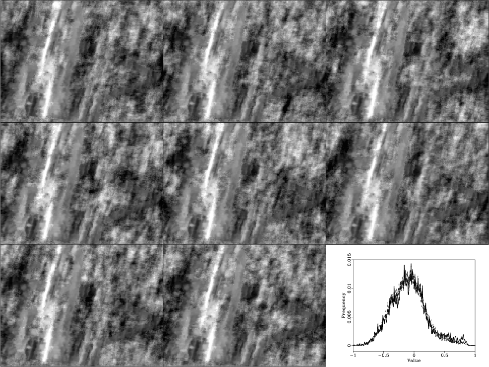
Figure 7 shows eight different realizations with a random noise level calculated through equation (8). Note how we have done a good job emulating the distribution of the known data. Each image shows some similar features but also significant differences (especially note within the `V' portion of the known data).
|
|---|
|
movie
Figure 7. Eight different realizations of the SeaBeam interpolation problem and their histograms. Note how the realizations vary away from the known data points. |
|
|
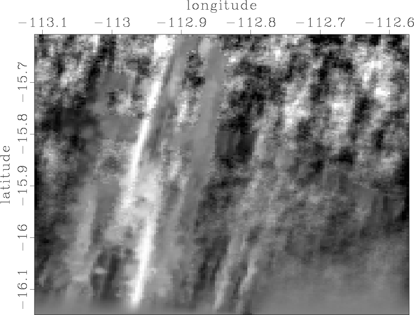
A potentially attractive feature of setting up the problem in this manner is that it easy to have both a space-varying covariance function (a steering filter or non-stationary PEF) along with a non-stationary variance. Figure 8 shows the SeaBeam example again with the variance increasing from left to right.
|
non-stat
Figure 8. Realization where the variance added to the image increases from left to right. |
|
|---|---|
|
|
|
|
|
|
Multiple realizations using standard inversion techniques |