Velocity continuation by spectral methods

Conclusions

I have applied two spectral methods for a numerical solution of the velocity continuation problem.

The Fourier method is attractive because of its numerical efficiency. However, it requires additional computational effort to suppress numerical artifacts: the inaccuracy of the grid transform and the artificial periodicity in the physical space.

The Chebyshev-$\tau$ method is free of most of these difficulties, although its overall efficiency can be slightly inferior to that of the Fourier method.

Both methods possess a ``spectral'' accuracy, which is highly desired if accuracy is a concern.

mig-impl
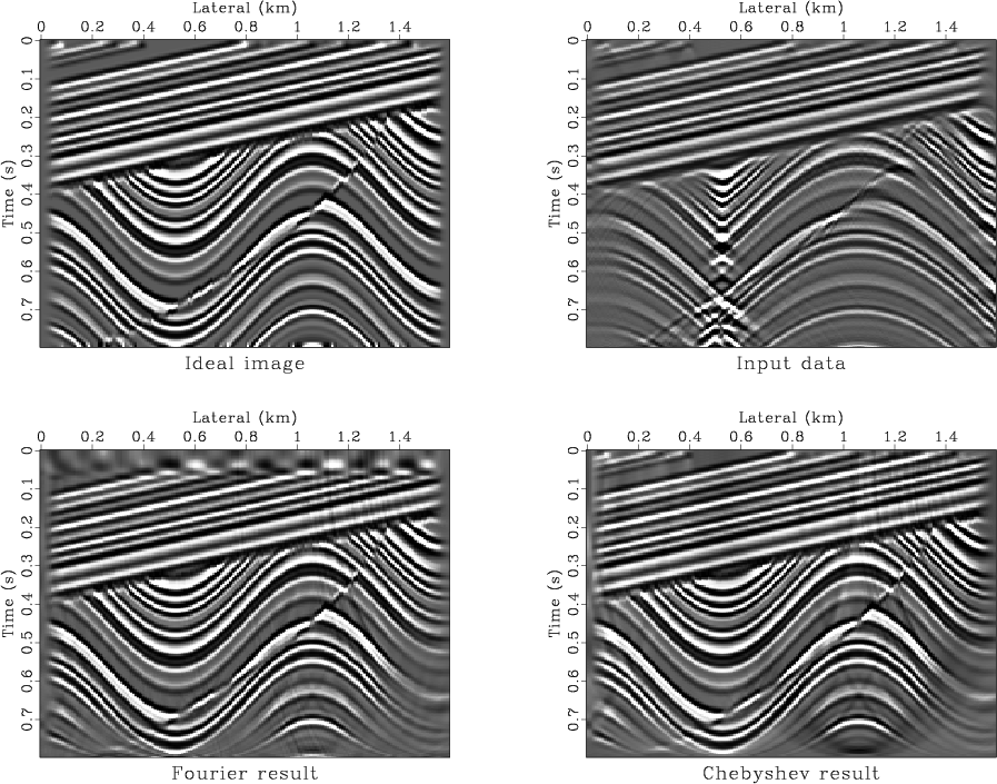
Figure 10. Top left: synthetic model (the ideal image). Top right: synthetic data. Bottom left: the result of velocity continuation with the Fourier method. Bottom right: the result of velocity continuation with the Chebyshev method.

Figure 10 compares the results of velocity continuation with different methods. The top left plot shows an implied subsurface model (an ``ideal image''). The top right plot is the corresponding synthetic data. The bottom left plot is the output of the Fourier method, and the bottom right plot is the output of the Chebyshev method. The Fourier result shows a poor quality in the shallow part (caused by subsampling in the $t^2$ grid). The wraparound artifacts were suppressed by a zero-padding correction. The quality of the Chebyshev result is noticeably higher. It is close to the best possible accuracy, under the natural limitations of seismic resolution.

Velocity continuation by spectral methods