|
|
|
|
A fast butterfly algorithm for generalized Radon transforms |
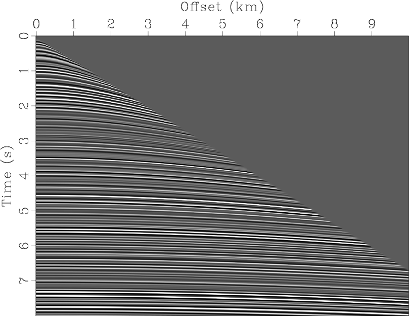
We now make two synthetic datasets using rectangular sampling ![]() ,
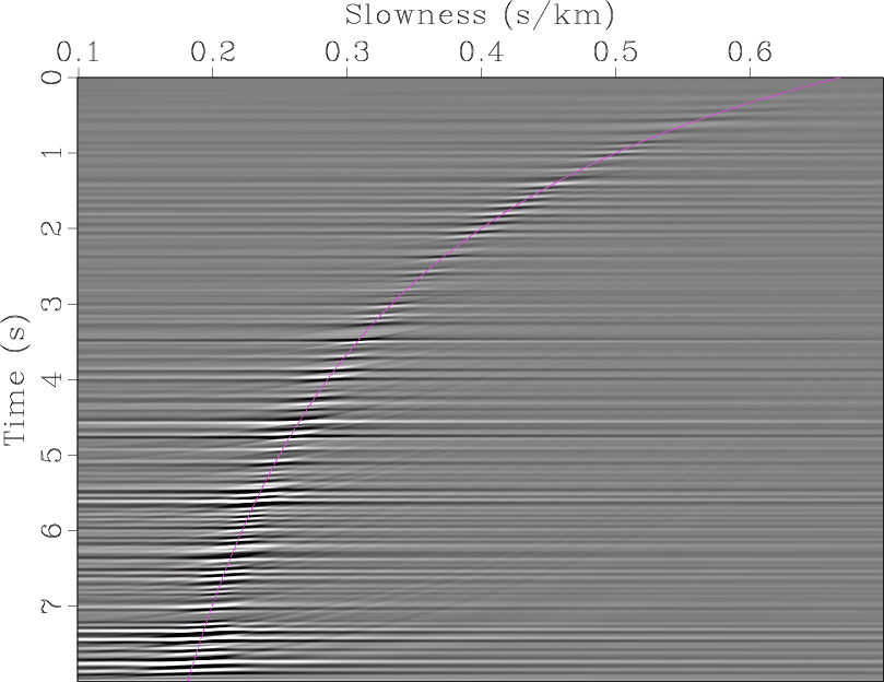
, ![]() . The first one (Figure 8) has the same range as the previous example (Figure 3), while the second one (Figure 9) doubles the range of time and offset. Results of the fast algorithm are shown in Figures 10 and 11. The purpose of showing these two examples is to demonstrate that the choice of
. The first one (Figure 8) has the same range as the previous example (Figure 3), while the second one (Figure 9) doubles the range of time and offset. Results of the fast algorithm are shown in Figures 10 and 11. The purpose of showing these two examples is to demonstrate that the choice of ![]() does not depend on the problem size, but rather on the range of parameters -- for the data in Figure 9, one has to increase
does not depend on the problem size, but rather on the range of parameters -- for the data in Figure 9, one has to increase ![]() to preserve the same accuracy (the range of
to preserve the same accuracy (the range of
![]() is about 125 for the first dataset, and 250 for the second one).
is about 125 for the first dataset, and 250 for the second one).

|
|---|
|
data-2
Figure 8. 2D synthetic CMP gather. |
|
|

|
|---|
|
data-3
Figure 9. 2D synthetic CMP gather. |
|
|

|
|---|
|
fmod-2
Figure 10. |
|
|

|
|---|
|
fmod-3
Figure 11. |
|
|
|
|
|
|
A fast butterfly algorithm for generalized Radon transforms |