Adaptive multiple subtraction using regularized nonstationary regression

Nonstationary deconvolution

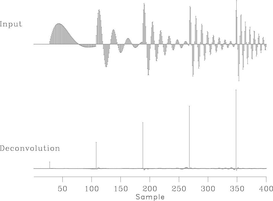
lpf
Figure 8. Benchmark test of nonstationary deconvolution from Claerbout (2008). Top: input signal, bottom: deconvolved signal using nonstationary regularized regression.

Figure 8 shows an application of regularized nonstationary regression to a benchmark deconvolution test from Claerbout (2008). The input signal is a synthetic trace that contains events with variable frequencies. A prediction-error filter is estimated by setting $N=2$, $s_1(x)=m(x-1)$ and $s_2(x)=m(x-2)$. I use triangle smoothing with a 5-sample radius as the shaping operator $\mathbf{S}$. The deconvolved signal (bottom plot in Figure 8) shows the nonstationary reverberations correctly deconvolved.

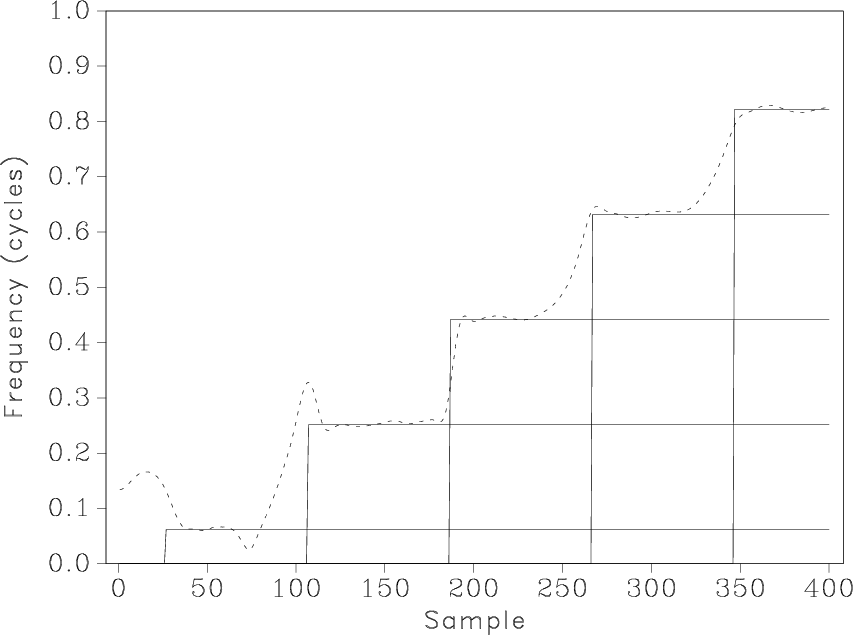
freq
Figure 9. Frequency of different components in the input synthetic signal from Figure 8 (solid line) and the local frequency estimate from non-stationary deconvolution (dashed line).

A three-point prediction-error filter $\{1,a_1,a_2\}$ can predict an attenuating sinusoidal signal

$$m(x) = \rho^x\,cos(\omega\,x)\;,$$ (8)

where $\omega$ is frequency, and $\rho$ is the exponent factor, provided that the filter coefficients are defined as

$$a_1 = -2\,\rho\,\cos(\omega)\;;$$ (9)

$$a_2 = \rho^2\;.$$ (10)

This fact follows from the simple identity

$$m(x)+a_1\,m(x-1)+a_2\,m(x-2) =$$

$$\rho^x\,\left[\cos(\omega\,x)-2\,\cos(\omega)\,\cos(\omega\,x-\omega)+\cos(\omega\,x-2\,\omega)\right] = 0\;.$$ (11)

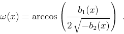
According to equations 9-10, one can get an estimate of the local frequency $\omega(x)$ from the non-stationary coefficients $b_1(x)=-a_1(x)$ and $b_2(x)=-a_2(x)$ as follows:

$$\omega(x) = \arccos\left(\frac{b_1(x)}{2\,\sqrt{-b_2(x)}}\right)\;.$$ (12)

Figure 9 shows frequency of the different components in the input non-stationary signal from Figure 8 and the local frequency estimate using equation 12. A reasonably accurate match between the true nonstationary frequencies and their estimate from nonstationary regression can be observed. The local frequency attribute (Fomel, 2007a) provides a different approach to the same problem.

Adaptive multiple subtraction using regularized nonstationary regression