|
|
|
|
A fast algorithm for 3D azimuthally anisotropic velocity scan |
Equation 10 is the discretized form of a 3D oscillatory integral of the type
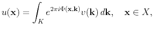 |
(11) |
The overall structure of the 3D butterfly algorithm basically follows its 2D analogue. The idea is to partition the computational domains ![]() and
and ![]() recursively into a pair of octrees,
recursively into a pair of octrees, ![]() and
and ![]() , ending at level
, ending at level ![]() (see Figure 1 for an illustration). Here
(see Figure 1 for an illustration). Here ![]() is chosen as an integer power of two, which is on the order of the maximum of
is chosen as an integer power of two, which is on the order of the maximum of
![]() for all possible
for all possible
![]() and
and
![]() (so it is mainly determined by the range of variables
(so it is mainly determined by the range of variables ![]() and
and
![]() ). A crucial property of this structure is that at arbitrary level
). A crucial property of this structure is that at arbitrary level ![]() , the side lengths
, the side lengths ![]() of a box
of a box ![]() in
in ![]() and
and ![]() of a box
of a box ![]() in
in ![]() always satisfy
always satisfy
![]() . Then when
. Then when
![]() ,
,
![]() restricted in
restricted in ![]() and
and ![]() respectively, one can construct a low-rank, separated expansion for the kernel function
respectively, one can construct a low-rank, separated expansion for the kernel function
![]() (via a Chebyshev interpolation):
(via a Chebyshev interpolation):

|
|---|
|
cube
Figure 1. Butterfly tree structure for the special case of |
|
|
Considering the initial Fourier transform for preparing data in ![]() domain, the overall complexity of our algorithm is roughly
domain, the overall complexity of our algorithm is roughly
![]() (
(
![]() terms are due to low-rank approximations, and
terms are due to low-rank approximations, and
![]() is bigger than
is bigger than
![]() ).
).
By comparison, the conventional straightforward velocity scan requires at least
![]() computations, which may quickly become a bottleneck as the problem size increases. Yet the efficiency of our algorithm is controlled mainly by
computations, which may quickly become a bottleneck as the problem size increases. Yet the efficiency of our algorithm is controlled mainly by
![]() with an
with an ![]() -dependent constant, where
-dependent constant, where ![]() is determined by the degree of oscillations in the kernel
is determined by the degree of oscillations in the kernel
![]() . Generally speaking,
. Generally speaking, ![]() depends on the maximum frequency and offset in the dataset, and the range of parameters in the model space. In practice,
depends on the maximum frequency and offset in the dataset, and the range of parameters in the model space. In practice, ![]() can often be chosen smaller than the grid size.
can often be chosen smaller than the grid size.
The significance of above analysis for the fast algorithm lies in the fact that the input and output data sizes ![]() and
and
![]() have little impact on the final computational cost; a dense sampling therefore becomes affordable.
have little impact on the final computational cost; a dense sampling therefore becomes affordable.
|
|
|
|
A fast algorithm for 3D azimuthally anisotropic velocity scan |
