A fast algorithm for 3D azimuthally anisotropic velocity scan

Example 2

We now further investigate the properties of the fast algorithm using a more realistic 3D synthetic CMP gather (Figure 4). The semblance plot computed by the fast algorithm is shown in Figure 5. Figure 6a is the isotropically NMO corrected data. After residual moveout using picked velocities from the semblance, curved events are flattened to the right position (Figure 6b).

We next fix $N_t=N_{\tau}=1000$ , $N_x=N_y=400$ and compare CPU time of the fast algorithm and the direct velocity scan for different $N_{W_{\cos}}$ and $N_{W_{\sin}}$ (Table 2). When $N_{W_{\cos}}$ and $N_{W_{\sin}}$ increase by a factor of 2, computation time of the direct velocity scan increases nearly by a factor of 4, which is consistent with our previous discussion on numerical complexity. On the other hand, CPU time of the fast algorithm is not affected much by the size of output sampling, again confirming our expectations.

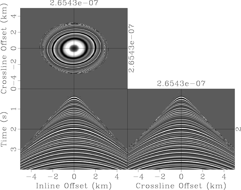
data
Figure 4. 3D synthetic CMP gather. $N_t=1000$ , $N_x=N_y=400$ . $\Delta t=0.004$ s, $\Delta x=\Delta y=25$ m.

Table: CPU time of direct velocity scan and fast butterfly algorithm for different $N_{W_{\cos}}$ and $N_{W_{\sin}}$ applied to the synthetic data in Figure 4.

	Direct	Fast butterfly	Speedup
$N_{W_{\cos}}\times N_{W_{\sin}}$	velocity scan	algorithm	factor
$10\times 10$	1847 s	145 s	12.7
$20\times 20$	7394 s	146 s	50.6
$100\times 100$	$\sim$ 184700 s	159 s	$\sim$ 1162
$200\times 200$	$\sim$ 738800 s	196 s	$\sim$ 3769

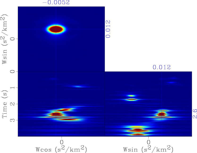
NMOsemb-1
Figure 5. Semblance plot computed by the fast algorithm. $N_{\tau }=1000$ , $N_{W_{\cos}}=N_{W_{\sin}}=200$ .

NMOdatacut,RMOdatacut
Figure 6. Synthetic gather (a) before and (b) after residual moveout using picked velocities from the semblance scan.

A fast algorithm for 3D azimuthally anisotropic velocity scan