Seislet transform and seislet frame

2-D data analysis with 2-D seislet frame

To show an example of 2-D data analysis with 2-D seislet frames, we use the CMP gather from Figure 7a. We try two different choices for selecting a set of dip fields for the frame construction.

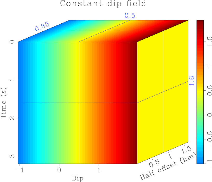
First, we define dip fields by scanning different constant dips (Figure 17a). In this case, the zero-scale coefficients out of the 2-D seislet frame correspond to the slant-stack (Radon transform) gather (Figure 18a). Figure 19a shows randomly selected example frame functions for the 2-D seislet frame using constant dips

Our second choice is a set of dip fields defined by the hyperbolic shape of seismic events on the CMP gather:

$$t(x)=\sqrt{t^2_0+\frac{x^2}{v^2}}\;,$$ (17)

where $t(x)$ is traveltime for reflection at offset $x$, $t_0$ is the zero-offset traveltime, and $v$ is the root-mean-square velocity. For a range of constant velocities, the direct relationship between dip and velocity is given by

$$p =\frac{dt}{dx}=\frac{x}{v^2 t}\;.$$ (18)

The dip field $p(x,t,v)$ is shown in Figure 17b. Analogously to the case of constant dips, the frame coefficients at the zero scale correspond to the hyperbolic Radon transform (Thorson and Claerbout, 1985), with the primary and multiple reflections distributed in different velocity ranges (Figure 18b). Figure 19b shows randomly selected frame functions for the 2-D seislet frame with varying dip fields defined by a range of constant velocities.

cdips,rrdips
Figure 17. Constant dip field (a) and time and space varying dip field (b).

cdiplet,rrdiplet
Figure 18. 2-D seislet frame coefficients with constant dip field (a) and with varying dip field (b).

cdipimps,rrdipimps
Figure 19. Randomly selected representative frame functions for 2-D seislet frame with constant dip field (a) and varying dip field (b).

Seislet transform and seislet frame