Azimuthally anisotropic 3D velocity continuation

Examples

Two simple synthetic examples are provided below to illustrate 3D velocity continuation over a range of velocity models. In the first example, we apply velocity continuation to a point diffractor. In the second example, we apply the method to a synthetic post-stack image of a set of faults. The second example illustrates fracture characterization through diffraction imaging as a potential application for 3D azimuthal velocity continuation. The data in both examples are modeled using equation 1, which geometrically approximates a diffraction surface as an elliptical-hyperbolic surface. Field data and more accurately modeled data will generally also exhibit nonhyperbolic moveout, for which equation 1 does not account. The physical validity and limitations of equation 1 are thoroughly discussed by Grechka and Tsvankin (1998), but we focus here on how well diffractions can be collapsed, and how well the velocity parameters can be measured, if the data are ideally described by equation 1.

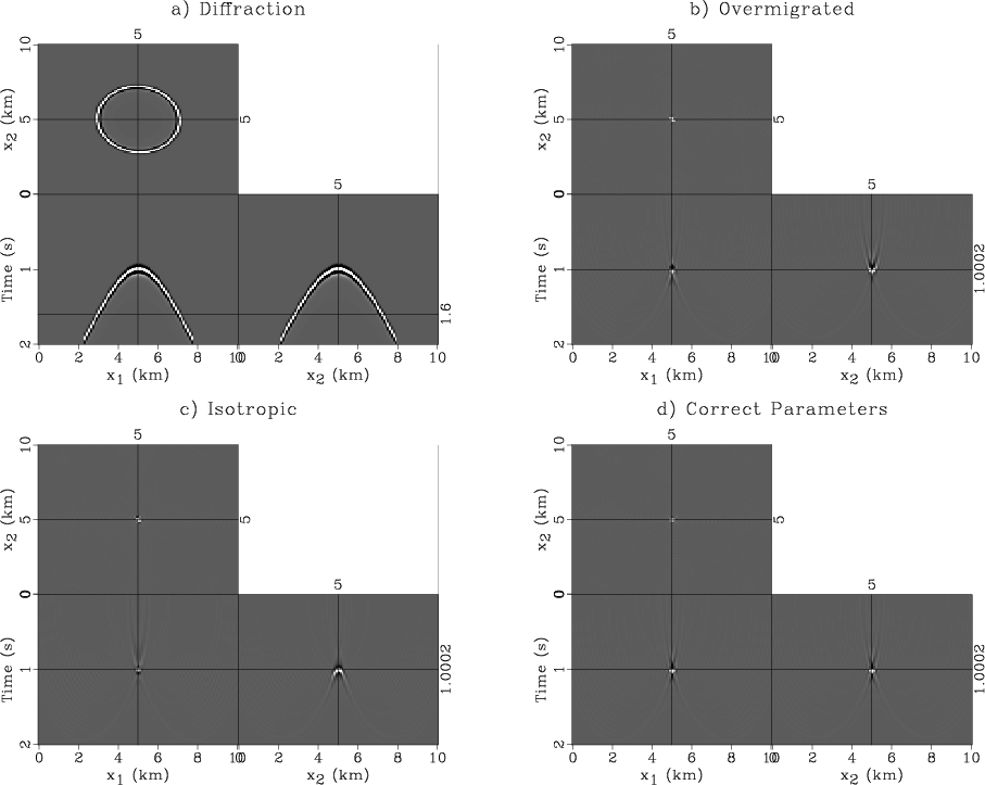
Figure 1a shows a single diffraction event, modeled using equation 1. The fastest direction of propagation is at $\beta$=105$^{\circ }$ counter-clockwise from the $x_1$ axis, with $V_{fast}$=3.50 km/s. The data in Figure 1a were modeled with $\sigma$=7% anisotropy, which may be quite high for most field cases, but it was chosen to allow the azimuthal variations in diffraction moveout to be visibly pronounced. As described above, we first stretch the time axis from $t$ to $\tilde{t}$ and take the 3D Fourier transform of the data. Then we apply the phase-shift prescribed by equation 18 for a range of $\tensor{W}$. We found it more intuitive to specify the parameter ranges in terms of $V_{x_1}$, $\beta$, and $\sigma$, and then convert them at each step into the three parameters of $\tensor{W}$ for use in equation 18. The inverse of the in-line velocity squared $1/V_{x_1}^2$ is equivalent to $W_{11}$, which, along with a given fast azimuth $\beta$ and percent anisotropy $\sigma$, can be used to calculate $W_{12}$ and $W_{22}$ using equations 3-5. Last, we apply the 3D inverse Fourier transform and unstretch from $\tilde{t}$ to $t$ to obtain the 6D image volume. Examples from the image volume using incorrect parameters are shown in Figures 1b-1c. The correct parameters are used in Figure 1d, where the image is well-focused.

images
Figure 1. (a) A single azimuthally anisotropic diffraction. (b) The diffraction migrated by velocity continuation using correct parameters except $\sigma$=10, resulting in overmigration along $x_2$. (c) Migration using the correct $W_{11}$, but assuming isotropy. The result is now undermigrated along $x_2$. (d) Migration using correct parameters. The image is well focused in both directions.

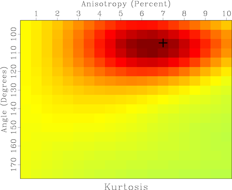
Since only a single diffraction is present in this example, we can measure kurtosis over a window spanning the entirety of each 3D image, reducing the kurtosis volume from 6D to 3D. Figure 2 is a 2D slice of the kurtosis volume at the correct $W_{11}=1/V_{x_1}^2$ value of 0.0935 = 1/(3.27 km/s)$^2$. The peak of the kurtosis map is near the correct values of $\sigma$=7 and $\beta$=105$^{\circ }$. Once the peak of the kurtosis map is identified, one could refine the increments around the peak to yield more accurate estimates. The physical limitations of resolving azimuthal velocity parameters are discussed by Al-Dajani and Alkhalifah (2000).

In practice, a conventional in-line 2D velocity analysis directly yields $W_{11}$ from $1/V_{x_1}^2$, so Figure 2 could illustrate a realistic scenario for using 3D velocity continuation to improve upon a previous isotropic velocity model. In such a case, one would use previous $V_{x_1}$ picks to hold $W_{11}$ constant, and then effectively test a variety of $W_{12}$ and $W_{22}$ values. Since $W_{11}$ and $W_{22}$ are measured with respect to the survey coordinates, either (or both) can be measured independently via a single-azimuth semblance scan, along $x_1$ or $x_2$, respectively. The best isotropic velocity based on a fully multiazimuth semblance scan will generally not represent either $W_{11}$ or $W_{22}$, but it can help limit the range of test parameters. Note that our method does not require prior knowledge of the velocity model, but without prior knowledge, the kurtosis measure remains a 6D volume. Although more difficult to visualize, the 6D kurtosis volume is computationally just as easily scanned for optimal imaging parameters as the 2D map in Figure 2.

focus
Figure 2. Kurtosis values for the velocity continuation of the diffraction in Figure 1a. The map covers a range of anisotropy and angle values with an increment in $\beta$ of 5$^{\circ }$ and an increment in $\sigma$ of 0.5%. The correct values at 105$^{\circ }$ and 7% anisotropy (indicated by crosshairs) coincide with the peak of the kurtosis map.

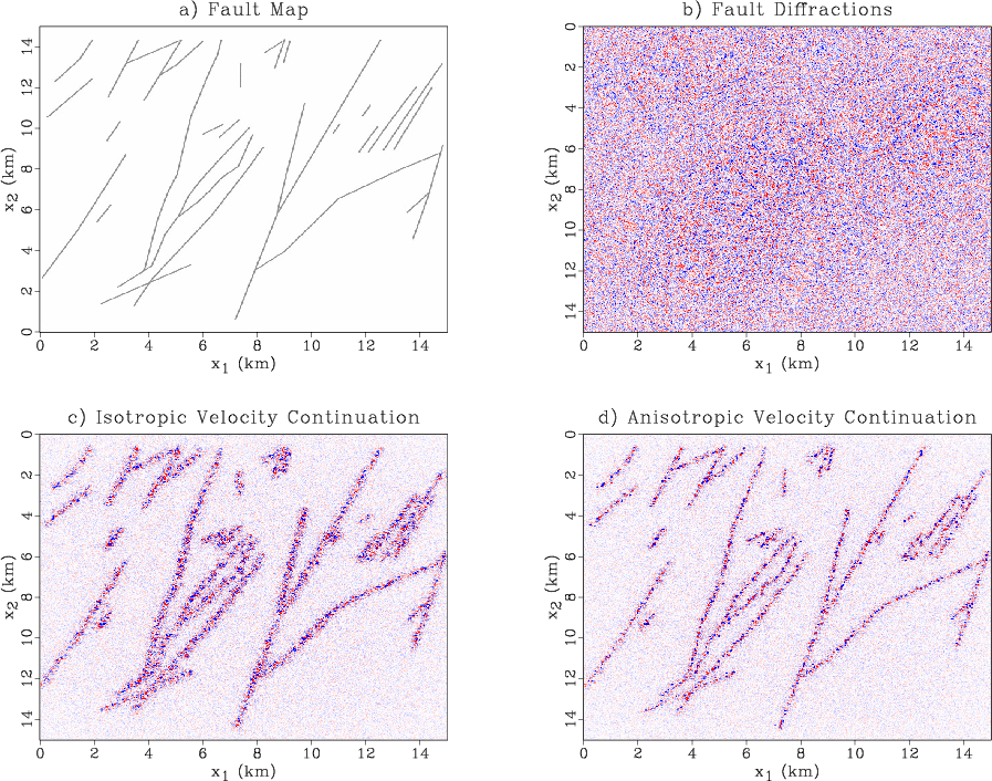
In the next example, we illustrate the concept of applying 3D anisotropic velocity continuation to diffraction imaging and fracture characterization. Figure 3a shows a 3D synthetic post-stack diffraction data set, equivalent to the ideal separation of diffractions from specular reflections in post-stack data following Fomel et al. (2007). A fault map from Hargrove (2010) (shown in Figure 3a) was digitized and used to create a 3D fracture model. Each fault location was used to generate a point diffraction in a homogeneous anisotropic background via equation 1. A timeslice of the modeled diffraction data is shown in Figure 3b. The faults in the model typically have a strike of 112$^{\circ }$, and in cases where faults and nearby fractures (which more likely influence the seismic velocity) are similarly aligned, the fast direction of seismic wave propagation tends to align with their strike. By assuming a typical tight sandstone velocity of $V_{fast}$=4.0 km/s with 3% anisotropy, we choose the modeling $\tensor{W}$ to be comprised of $W_{11}$=0.0659, $W_{22}$=0.0631, and $W_{12}$=0.0014 (all in s$^2$/km$^2$). This results in a fast velocity direction along the strike of the faults. In Figure 3d, we see that 3D velocity continuation using the correct parameters (again found by maximum kurtosis) allows the faults to be clearly imaged. If an intermediate isotropic velocity model is used, as in Figure 3c, the diffractions are still imaged, but they are not as well-focused compared to the anisotropically migrated diffractions in Figure 3d. Conventionally, diffraction arrivals such as those in Figure 3a may be viewed as noise, but by separating them and treating them as signal, we can see here that imaging of steep and detailed features while simultaneously extracting anisotropy information may be possible.

images-mig-all
Figure 3. (a) Fault map from Northwest Scotland (Hargrove, 2010) used to model diffraction data. (b) Synthetic post-stack diffraction data modeled using equation 1 and a 3D model based on the fault map in (a). (c) Diffractions from (b) migrated using an isotropic velocity model. (d) Diffractions from (b) migrated by anisotropic 3D velocity continuation.

Azimuthally anisotropic 3D velocity continuation