Acoustic Staggered Grid Modeling in IWAVE

PML Effectiveness

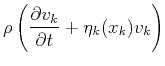
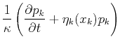
The IWAVE acoustic staggered grid scheme implements the Perfectly Matched Layer (PML) approach to absorbing boundary conditions, in one of the simpler of its many guises (a split field approach - (Hu et al., 2007)). After some manipulation, the acoustic PML system for the physical velocity ${\bf v}$ and an artificial vector pressure ${\bf p}$ takes the form

$$\rho \left(\frac{\partial v_k}{\partial t} + \eta_k(x_k)v_k\right) = - \frac{\partial p_k}{\partial x_k},$$

$$\frac{1}{\kappa}\left(\frac{\partial p_k}{\partial t} + \eta_k(x_k)p_k\right) = -\nabla \cdot {\bf v} + g$$ (3)

in which the $k$th component of the attenuation profile vector ${\bf\eta}$ depends only on $x_k$, and can be stored as a collection of 1D objects. Ordinary acoustic wave propagation takes place where ${\bf\eta}={\bf0}$, and if the components of the vector pressure ${\bf p}$ are all the same in this zone, then they remain the same there, and any one of them may be regarded as the same as the physical pressure field. Outside of the physical domain, where waves are to be attenuated, ${\bf {\eta}}$ should ibe positive; at the boundary of the physical domain, it should vanish to positve order. We elected to make ${\bf {\eta}}$ cubic in distance to the boundary: for a PML layer of width $L_{k,r}$, beginning at $x_k=x_{k,r}$ along the $k$th coordinate axes,

$$\eta(x_k) = \eta_0 \left(\frac{x_k-x_{k,r}}{L_{k,r}}\right)^3$$

Thus there are four PML boundary layer thicknesses in 2D, six in 3D, one for each side of the simulation cube. The IWAVE convention imposes pressure-free boundary conditions on the exterior boundary of the PML domain. Thus $L=0$ signifies a free surface boundary face. Any face of the boundary may be assigned a zero-pressure condition ($L=0$) or a PML zone of any width ($L>0$).

Many implementations of PML, especially for elasticity, confine the extra PML fields (in this case, the extra pressure variables) to explicitly constructed zones around the boundary, and use the standard physical system in the domain interior. We judged that for acoustics little would be lost in either memory or efficiency, and much code bloat avoided, if we were to solve the system (3) in the entire domain.

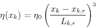
Considerable experience and some theory (Moczo et al., 2006; Hu et al., 2007) suggest that the system 3 will effectively absorb waves that impinge on the boundary, emulating free space in the exterior of the domain, if the PML zones outside the physical domain in which ${\bf {\eta}}$ are roughly a half-wavelength wide, and $\eta_0=0$.

A simple 2D example illustrates the performance of this type of PML. The physical domain is a 1.8 x 7.6 km; the same domain is used in the experiments reported in the next section. A point source is placed at $z$=40 m, $x=3.3$ km, with a Gaussian derivative time dependence with peak amplitude at about 5 Hz, and signifcant energy at 3 Hz but little below. The acoustic velocity is 1.5 km/s throughout the domain, so the effective maximum wavelength is roughly 500 m. The density is also constant, at 1 g/${\rm cm}^3$. A snapshot of the wavefield at 1.2 s after source onsiet (Figure 1), before the wave has reached the boundary of the domain, shows the expected circular wavefront. At 4.0 s, a simulation with zero-pressure boundary conditions on all sides of the physical domain produces the expected reflections, Figure 2. With PML zones of 250 m on the bottom and sides of the domain, so that only the top is a zero-pressure surface, and $\eta_0=1$, the wave and its free-surfacec ghost both appear to leave the domain (Figure 3, plotted on the same grey scale). The maximum amplitude visible in Figure 2 is roughly $7.1 \times 10^{-2}$, whereas the maximum amplitude in Figure 3 is $7.0 \times 10^{-5}$. The actual reflection coefficient is likely less than $10^{-3}$, as the 2D free space field does not have a lacuna behind the wavefront, but decays smoothly, so the low end of the wavelet spectrum remains.

It is not possible to decrease the PML layer thickness much beyond the nominal longest half-wavelength and enjoy such small reflections. Figure 4 shows the field at 4.0 s with PML zones of width 100 m on bottom and sides, and an apparently optimal choice of $\eta_0$. The maximum amplitude is $2.3 \times 10^{-4}$, and a reflected wave is clearly visible at the same grey scale.

Acoustic Staggered Grid Modeling in IWAVE