 |
 |
 |
 | A numerical tour of wave propagation |  |
![[pdf]](icons/pdf.png) |
Next: Conjugate gradient (CG) implementation
Up: Full waveform inversion (FWI)
Previous: Full waveform inversion (FWI)
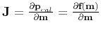
In terms of Eq. (64),
![\begin{displaymath}\begin{split}\frac{\partial E(\textbf{m})}{\partial m_i} &=\f...
...^{\dagger}\Delta \textbf{p}\right], i=1,2,\ldots,M. \end{split}\end{displaymath}](img199.png) |
(71) |
That is to say,
![$\displaystyle \nabla E_{\textbf{m}}=\nabla E(\textbf{m})=\frac{\partial E(\text...
...textbf{p}\right] =\mathtt{Re}\left[\textbf{J}^{\dagger}\Delta \textbf{p}\right]$](img200.png) |
(72) |
where
 takes the real part, and
 is the Jacobian matrix, i.e., the sensitivity or the Fréchet derivative matrix.
Differentiation of the gradient expression (71) with respect to the model parameters gives the following expression for the Hessian
 :
:
![\begin{displaymath}\begin{split}\textbf{H}_{i,j}&=\frac{\partial^2 E(\textbf{m})...
...frac{\partial\textbf{p}_{cal}}{\partial m_j}\right] \end{split}\end{displaymath}](img203.png) |
(73) |
In matrix form
![$\displaystyle \textbf{H}=\frac{\partial^2 E(\textbf{m})}{\partial \textbf{m}^2}...
...(\Delta \textbf{p}^*, \Delta \textbf{p}^*, \ldots, \Delta \textbf{p}^*)\right].$](img204.png) |
(74) |
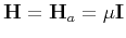
In many cases, this second-order term is neglected for nonlinear inverse problems. In the following, the remaining term in the Hessian, i.e.,
![$ \textbf{H}_a=\mathtt{Re}[\textbf{J}^{\dagger}\textbf{J}]$](img205.png) , is referred to as the approximate Hessian. It is the auto-correlation of the derivative wavefield. Eq. (68) becomes
, is referred to as the approximate Hessian. It is the auto-correlation of the derivative wavefield. Eq. (68) becomes
![$\displaystyle \Delta \textbf{m} =-\textbf{H}^{-1}\nabla E_{\textbf{m}} =-\textbf{H}_a^{-1}\mathtt{Re}[\textbf{J}^{\dagger}\Delta \textbf{p}].$](img206.png) |
(75) |
The method which solves equation (74) when only
 is estimated is referred to as the Gauss-Newton method. To guarantee th stability of the algorithm (avoiding the singularity), we can use
 , leading to
![$\displaystyle \Delta \textbf{m} =-\textbf{H}^{-1}\nabla E_{\textbf{m}} =-(\text...
... \textbf{I})^{-1}\mathtt{Re}\left[\textbf{J}^{\dagger}\Delta \textbf{p}\right].$](img209.png) |
(76) |
Alternatively, the inverse of the Hessian in Eq. (68) can be replaced by
 , leading to the gradient or steepest-descent method:
![$\displaystyle \Delta \textbf{m} =-\mu^{-1}\nabla E_{\textbf{m}} =-\alpha\nabla ...
...a\mathtt{Re}\left[\textbf{J}^{\dagger}\Delta \textbf{p}\right],\alpha=\mu^{-1}.$](img211.png) |
(77) |
At the  -th iteration, the misfit function can be presented using the 2nd-order Taylor-Lagrange expansion
 |
(78) |
Setting
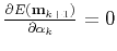 gives
gives
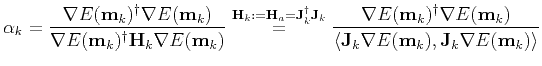 |
(79) |
|
|
|
|
| A numerical tour of wave propagation | |
|
Next: Conjugate gradient (CG) implementation
Up: Full waveform inversion (FWI)
Previous: Full waveform inversion (FWI)
2021-08-31