 |
 |
 |
 | A numerical tour of wave propagation |  |
![[pdf]](icons/pdf.png) |
Next: Gradient computation
Up: Full waveform inversion (FWI)
Previous: Conjugate gradient (CG) implementation
Recall that the basic acoustic wave equation can be specified as
 |
(91) |
where
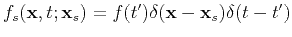 .
The Green's function
.
The Green's function
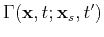 is defined by
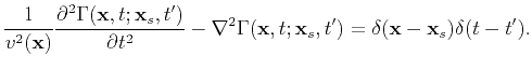 |
(92) |
Thus the integral representation of the solution can be given by
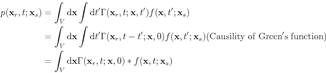 |
(93) |
where  denotes the convolution operator.
A perturbation
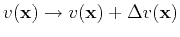 will produce a field
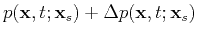 defined by
![$\displaystyle \frac{1}{(v(\textbf{x})+\Delta v(\textbf{x}))^2}\frac{\partial^2 ...
...xtbf{x}_s)+\Delta p(\textbf{x},t;\textbf{x}_s)] =f_s(\textbf{x},t;\textbf{x}_s)$](img240.png) |
(94) |
Note that
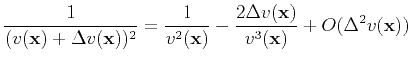 |
(95) |
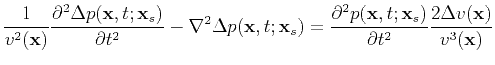
Eq. (94) subtracts Eq. (91), yielding
![$\displaystyle \frac{1}{v^2(\textbf{x})}\frac{\partial^2 \Delta p(\textbf{x},t;\...
...x},t;\textbf{x}_s)]}{\partial t^2}\frac{2\Delta v(\textbf{x})}{v^3(\textbf{x})}$](img242.png) |
(96) |
Using the Born approximation, Eq. (96) becomes
 |
(97) |
Again, based on integral representation, we obtain
 |
(98) |
|
|
|
|
| A numerical tour of wave propagation | |
|
Next: Gradient computation
Up: Full waveform inversion (FWI)
Previous: Conjugate gradient (CG) implementation
2021-08-31