GEO 365N/384S Seismic Data Processing Computational Assignment 5

Parabolic Radon transform

In this part of the assignment, we will process the Viking Graben data to attenuate multiple reflections using the parabolic Radon transform.

1. Change directory to hw5/pradon.
2. Run

   scons -c
   

   to remove (clean) previously generated files.
3. We start by picking from the previous processing steps: applying deconvolution and surface-consistent amplitude corrections to prepare data for further processing. To go through these steps and to display the resultant CMP gathers, run

   scons cmps.view
   

   You can also improve the results using your work from Assignment 4.

   

   vscan1
   Figure 4. Initial velocity analysis. From left to right: selected CMP gather, gather after muting first arrivals, semblance scan with the picked primary velocity trend.

   

   
   

4. We will select one CMP gather to test our multiple-attenuation strategy. Figure 4 shows the selected CMP gather and the result of velocity analysis by semblance scanning. To reproduce it on your screen, run

   scons vscan1.view
   

   As evident from the semblance scan, the gather is heavily contaminated by multiples, including water-layer multiples and surface-related peglegs. For further processing, we will attempt to pick the primary velocity trend, using muting and automatic picking.

   

   parab
   Figure 5. Applying the parabolic Radon transform. From left to right: NMO using the picked velocity trend, parabolic Radon transform, data reconstructed by the inverse transform.

   

   
   

5. Applying the normal moveout (NMO) with the picked primary trend makes primary reflections nearly flat and multiple reflections curved (parabolic). Now the data are ready for transformation by the parabolic Radon transform. The results are shown in Figure 5. To reproduce it on your screen, run

   scons parab.view
   

   As with the linear Radon, the transform is implemented in the temporal Fourier domain and makes use of the Toeplitz structure to accelerate least-squares inversion.

   

   cut
   Figure 6. Isolating signal in the parabolic Radon domain. From left to right: parabolic Radon transform, isolated nearly-flat events, signal reconstructed by the inverse transform.

   

   
   

6. Next, we isolate primary events by making a cut in the parabolic Radon domain to separate events with small curvature (Figure 6). To display the result on your screen, run

   scons cut.view
   

   

   primary,pvscan1
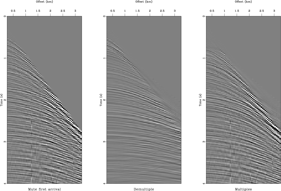
   Figure 7. Separating signal (primary reflections) and noise (multiple reflections). (a) From left to right: input CMP gather, estimated primaries, estimated multiples. (b) Velocity analysis using semblance scan. From left to right: using all data, using estimated primaries, using estimated multiples.

   

   
   

7. To go back to the CMP domain requires applying the inverse NMO. The final result of separating primaries from multiples is shown in Figure 7a. We can verify the separation by running the semblance scan on the separated events (Figure 7b.) To reproduce these figures on your screen, run

   scons primary.view pvscan1.view
   

8. Your task, as before, is to try improving the separation result. There are several possible steps to modify:
   • picking the primary trend
   • parameters of the parabolic Radon transform
   • separating primary events in the parabolic Radon domain

9. (EXTRA CREDIT) For an extra credit, apply the procedure to all CMP gathers in the Viking Graben data and generate an improved stacked section.

from rsf.proj import *

# Download Viking Graben data
Fetch('seismic.segy','viking')
#Fetch('seismic.segy','VikingGrabbenLine12',
#      top='/home/p1/seismic_datasets/SeismicProcessingClass',
#      server='local')

# Convert from SEGY to RSF
Flow('viking tviking viking.asc viking.bin','seismic.segy',
     '''
     segyread tfile=${TARGETS[1]} 
     hfile=${TARGETS[2]} bfile=${TARGETS[3]}
     ''')

# Far-field wavelet
Fetch('FarField.dat','Mobil_Avo_Viking_Graben_Line_12',
      top='open.source.geoscience/open_data',
      server='http://s3.amazonaws.com')

# Convert from ASCII to RSF
Flow('wavelet','FarField.dat',
     '''
     echo in=$SOURCE data_format=ascii_float n1=500 o1=0 d1=0.0008 
     label1=Time unit1=s n2=1 | dd form=native
     ''')

# Subsample to data sampling
Flow('wavelet4','wavelet','window j1=5 | pad n1=1500')

prog = Program('convolve.c')
convolve = str(prog[0])

# Estimate PEF by iterative least-squares inversion
Flow('filter0',None,'spike n1=100 k1=1')
Flow('filter',['wavelet4',convolve,'filter0'],
     '''
     conjgrad ./${SOURCES[1]} nf=100 data=${SOURCES[0]}
     niter=100 mod=${SOURCES[2]} 
     ''')

# Wavelet deconvolution
Flow('wdecon',['filter','wavelet4',convolve],
     '''
     ./${SOURCES[2]} data=${SOURCES[1]} adj=n | 
     add ${SOURCES[1]} scale=-1,1 | window n1=100
     ''')

# Process all traces
Flow('decon',['filter','viking',convolve],
     '''
     ./${SOURCES[2]} data=${SOURCES[1]} adj=n | 
     add ${SOURCES[1]} scale=-1,1
     ''')

# Average trace amplitude
Flow('arms','decon',
     'mul $SOURCE | stack axis=1 | math output="log(input)" ')

# shot/offset indeces: fldr and tracf
Flow('index','tviking','window n1=2 f1=2 | transp')

Flow('fldr tracf scarms','arms index',
     '''
     sc index=${SOURCES[1]} out2=${TARGETS[1]} pred=${TARGETS[2]} 
     niter=10
     ''')

# Apply to all traces

Flow('ampl','scarms',
     '''
     math output="exp(-input/2)" | 
     spray axis=1 n=1500 d=0.004 o=0
     ''')
Flow('adecon','decon ampl','mul ${SOURCES[1]}')

# Convert to CDP gathers, time-power gain 
Flow('cmps','adecon',
     '''
     intbin xk=cdpt yk=cdp | window max1=4 | 
     pow pow1=2 
     ''')

Result('cmps',
       '''
       byte gainpanel=all | transp plane=23 memsize=5000 |
       grey3 frame1=750 frame2=1000 frame3=20 
       point1=0.8 point2=0.8
       title="CMP Gathers" label2="CMP Number" 
       ''')
    
# Extract offsets
Flow('offsets mask','tviking',
     '''
     headermath output=offset | 
     intbin head=$SOURCE xk=cdpt yk=cdp mask=${TARGETS[1]} | 
     dd type=float |
     scale dscale=0.001
     ''')

# Extract one CMP gather
########################

Flow('mask1','mask','window n3=1 f3=1200 squeeze=n')
Flow('cmp','cmps mask1',
     'window n3=1 f3=1200 | headerwindow mask=${SOURCES[1]}')
Plot('cmp','grey title="CMP gather" clip=8.66')

Flow('offset','offsets mask1',
     '''
     window n3=1 f3=1200 squeeze=n | 
     headerwindow mask=${SOURCES[1]}
     ''')

# Mute 
Flow('mute','cmp',
     '''
     reverse which=2 | put label2=Offset unit2=km o2=0.287 d2=0.05 | 
     mutter half=n v0=1.2
     ''')
Plot('mute','grey title="Mute first arrival" clip=8.66')

# Velocity scan

Flow('vscan1','mute',
     '''
     vscan semblance=y half=n v0=1.2 nv=131 dv=0.02 
     ''')
Plot('vscan1',
     'grey color=j allpos=y title="Semblance scan" unit2=km/s')

# Automatic pick

Flow('vpick1','vscan1',
     '''
     mutter inner=y x0=1.4 half=n v0=0.45 t0=0.5 | 
     pick rect1=50 vel0=1.5
     ''')
Plot('vpick1',
     '''
     graph yreverse=y transp=y plotcol=7 plotfat=7 
     pad=n min2=1.2 max2=3.8 wantaxis=n wanttitle=n
     ''')

Plot('vscan2','vscan1 vpick1','Overlay')

Result('vscan1','cmp mute vscan2','SideBySideAniso')

Flow('nmo','mute vpick1','nmo half=n velocity=${SOURCES[1]}')
Plot('nmo','grey title="NMO with primary velocity" ')

# Parabolic Radon transform

Flow('radon','nmo',
     'radon adj=y spk=n parab=y p0=-0.1 dp=0.002 np=151')
Plot('radon',
     '''
     grey title="Parabolic Radon transform" 
     label2=Curvature unit2="s/km2_" 
     ''')

Flow('inv','radon','radon adj=n parab=y nx=60 dx=0.05 ox=0.287')
Plot('inv',
     'grey title="Inverse parabolic Radon transform" clip=8.66')

Result('parab','nmo radon inv','SideBySideAniso')

qmin=0.01 # minimum curvature for noise
tmin=0.75 # minimum time for noise

Flow('cut','radon','cut min2=%g min1=%g' % (qmin,tmin))
Plot('cut',
     '''
     grey title="Radon transform cut" 
     label2=Curvature unit2="s/km2_" 
     ''')

Flow('signal','cut','radon adj=n parab=y nx=60 dx=0.05 ox=0.287')
Plot('signal','grey title="Radon transform signal" ')

Result('cut','radon cut signal','SideBySideAniso')

# Apply inverse NMO

Flow('primary','signal vpick1',
     'inmo half=n velocity=${SOURCES[1]}')
Plot('primary','grey title="Demultiple" clip=8.66')

Flow('multiples','mute primary','add scale=1,-1 ${SOURCES[1]}')
Plot('multiples','grey title="Multiples" clip=8.66')

Result('primary','mute primary multiples','SideBySideAniso')

# Velocity scan

Flow('pvscan1','primary',
     '''
     vscan semblance=y half=n v0=1.2 nv=131 dv=0.02 
     ''')
Plot('pvscan1',
     'grey color=j allpos=y title="Primary semblance scan" ')

Flow('mvscan1','multiples',
     '''
     vscan semblance=y half=n v0=1.2 nv=131 dv=0.02 
     ''')
Plot('mvscan1',
     'grey color=j allpos=y title="Multiples semblance scan" ')

Result('pvscan1','vscan1 pvscan1 mvscan1','SideBySideAniso')

End()

GEO 365N/384S Seismic Data Processing Computational Assignment 5