Homework 2

Running median and running mean filters

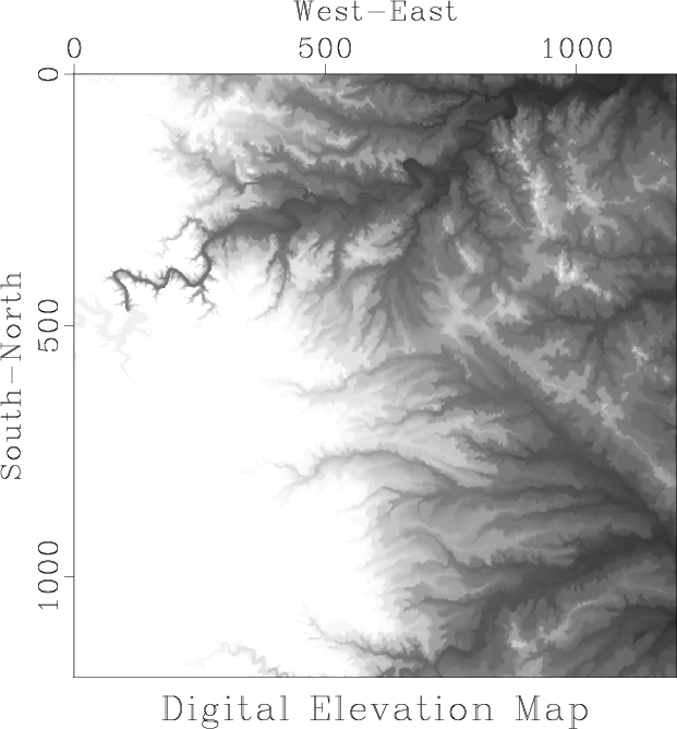
dem Figure 2. Digital elevation map of the west Austin area.

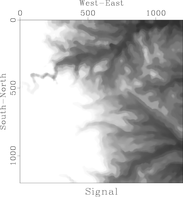
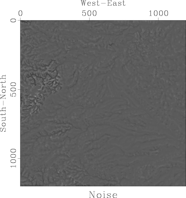
In this part of the homework, we will analyze the digital elevation map of the West Austin Area, shown in Figure 2. Our task is to separate the data into ``signal'' and ``noise'' by applying running mean and median filters. The result of applying a running median filter is shown in Figure 3. Running median effectively smooths the data by removing local outliers.

ave,res
Figure 3. Data separated into signal (a) and noise (b) by applying a running median filter.

The algorithm is implemented in program running.c.

/* Apply running mean or median filter */

#include <rsf.h>

static float slow_median(int n, float* list)
/* find median by slow sorting, changes list */
{
    int k, k2;
    float item1, item2;
    
    for (k=0; k < n; k++) {
	item1 = list[k];

	/* assume everything up to k is sorted */
        for (k2=k; k2 > 0; k2-) {
            item2 = list[k2-1];
            if (item1 >= item2) break;
	    list[k2]   = item2;
	}
	list[k2] = item1;
    }
    
    return list[n/2];
}

int main(int argc, char* argv[]) 
{
    int w1, w2, nw, s1,s2, j1,j2, i1,i2,i3, n1,n2,n3;
    char *what;
    float **data, **signal, **win;
    sf_file in, out;

    sf_init (argc,argv);
    in = sf_input("in");
    out = sf_output("out");

    /* get data dimensions */
    if (!sf_histint(in,"n1",&n1)) sf_error("No n1=");
    if (!sf_histint(in,"n2",&n2)) sf_error("No n2=");
    n3 = sf_leftsize(in,2);

    /* input and output */
    data = sf_floatalloc2(n1,n2);
    signal = sf_floatalloc2(n1,n2);

    if (!sf_getint("w1",&w1)) w1=5;
    if (!sf_getint("w2",&w2)) w2=5;
    /* sliding window width */

    nw = w1*w2;
    win = sf_floatalloc2(w1,w2);

    what = sf_getstring("what"); 
    /* what to compute 
       (fast median, slow median, mean) */
    if (NULL == what) what="fast";

    for (i3=0; i3 < n3; i3++) {

	/* read data plane */
	sf_floatread(data[0],n1*n2,in);
	
	for (i2=0; i2 < n2; i2++) {
	    s2 = SF_MAX(0,SF_MIN(n2-w2,i2-w2/2-1));
	    for (i1=0; i1 < n1; i1++) {
		s1 = SF_MAX(0,SF_MIN(n1-w1,i1-w1/2-1));

		/* copy window */
		for (j2=0; j2 < w2; j2++) {
		    for (j1=0; j1 < w1; j1++) {
			win[j2][j1] = data[s2+j2][s1+j1];
		    }}

		switch (what[0]) {
		    case 'f': /* fast median */
			signal[i2][i1] = 
			    sf_quantile(nw/2,nw,win[0]);
			break;
		    case 's': /* slow median */
			signal[i2][i1] = 
			    slow_median(nw,win[0]);
			break;
		    case 'm': /* mean */
		    default:
			/* !!! ADD CODE !!! */
			break;
		}
	    }
	}
	
	/* write out */
	sf_floatwrite(signal[0],n1*n2,out);
    }	

    exit(0);
}

1. Change directory to hw2/running.
2. Run

   scons view
   

   to reproduce the figures on your screen.
3. Modify the running.c program and the SConstruct file to compute running mean instead of running median. Compare the results.
4. EXTRA CREDIT for improving the efficiency of the running median algorithm. Run

   scons time.vpl
   

   to display a figure that compares the efficiency of running median computations using the slow sorting from function median in program running.c and the fast quantile algorithm (library function sf_quantile ). Your goal is to make the algorithm even faster. You may consider parallelization, reusing previous windows, other fast sorting strategies, etc.

from rsf.proj import *

# Download data
Fetch('austin-w.HH','bay')

# Convert format
Flow('dem','austin-w.HH','dd form=native')

# Display
def plot(title):
    return '''
    grey clip=250 allpos=y title="%s" 
    screenratio=1
    ''' % title

Result('dem',plot('Digital Elevation Map'))

# Running median program
run = Program('running.c')

w = 30

# !!! CHANGE BELOW !!!
Flow('ave','dem %s' % run[0],
     './${SOURCES[1]} w1=%d w2=%d what=fast' % (w,w))
Result('ave',plot('Signal'))

# Difference
Flow('res','dem ave','add scale=1,-1 ${SOURCES[1]}')
Result('res',plot('Noise') + ' allpos=n')

#############################################################

import sys

if sys.platform=='darwin':
     gtime = WhereIs('gtime')
else:
     gtime = WhereIs('gtime') or WhereIs('time')

if not gtime:
    print '''
For computing CPU time, please install GNU time!
    '''
     
# slow or fast
for case in ('fast','slow'):

    ts = []
    ws = []

    time = 'time-' + case
    wind = 'wind-' + case

    # loop over window size
    for w in range(3,16,2):
        itime = '%s-%d' % (time,w)
        ts.append(itime)

        iwind = '%s-%d' % (wind,w)
        ws.append(iwind)

        # measure CPU time


        Flow(iwind,None,'spike n1=1 mag=%d' % (w*w)) 
        Flow(itime,'dem %s' % run[0],
             '''
             ( (%s -f "%%S %%U"
             ./${SOURCES[1]} < ${SOURCES[0]} 
              w1=%d w2=%d what=%s > /dev/null ) 2>&1 )
              > time.out &&
             (tail -1 time.out; 
              echo in=time0.asc n1=2 data_format=ascii_float)
              > time0.asc &&
             dd form=native < time0.asc | stack axis=1 norm=n
             > $TARGET &&
             /bin/rm time0.asc time.out
             ''' % (gtime,w,w,case),stdin=0,stdout=-1)
        
    Flow(time,ts,'cat axis=1 ${SOURCES[1:%d]}' % len(ts))
    Flow(wind,ws,'cat axis=1 ${SOURCES[1:%d]}' % len(ws))

    # complex numbers for plotting
    Flow('c'+time,[wind,time],
         '''
         cat axis=2 ${SOURCES[1]} |
         transp |
         dd type=complex
         ''')

# Display CPU time
Plot  ('time','ctime-fast ctime-slow',
       '''
       cat axis=1 ${SOURCES[1]} | transp |
       graph dash=0,1 wanttitle=n
       label2="CPU Time" unit2=s
       label1="Window Size" unit1=
       ''',view=1)

End()

Homework 2