|
|
|
|
Signal and noise separation in prestack seismic data using velocity-dependent seislet transform |
We test VD-seislet denoising by employing a field land data provided
by Geofizyka Torun Sp. Z.o.o, Poland from FreeUSP
website![]() . Figure 9a
show the CMP gathers after removing most of ground roll. The strong
random noise makes reflection events hardly visible. However, velocity
analysis from equation 6 can still produce a reasonable
velocity field. Equation 7 converts RMS velocity to
seismic pattern (Figure 9b), which
displays the hyperbolic slopes from negative to positive in CMP
gathers and varying slopes in common-offset
section. VD-seislet transform utilizes the slopes to compress
reflections along offset
axis. Figure 9c shows the
VD-seislet coefficients, in which the small dynamic range of seislet
coefficients implies a good compression ratio. If we choose the
significant coefficients at the coarse scale, e.g., scale
. Figure 9a
show the CMP gathers after removing most of ground roll. The strong
random noise makes reflection events hardly visible. However, velocity
analysis from equation 6 can still produce a reasonable
velocity field. Equation 7 converts RMS velocity to
seismic pattern (Figure 9b), which
displays the hyperbolic slopes from negative to positive in CMP
gathers and varying slopes in common-offset
section. VD-seislet transform utilizes the slopes to compress
reflections along offset
axis. Figure 9c shows the
VD-seislet coefficients, in which the small dynamic range of seislet
coefficients implies a good compression ratio. If we choose the
significant coefficients at the coarse scale, e.g., scale ![]() 8, and
zero out difference coefficients at the finer scales, the inverse
transform effectively removes incoherent noise from the gathers
(Figure 9d).
8, and
zero out difference coefficients at the finer scales, the inverse
transform effectively removes incoherent noise from the gathers
(Figure 9d).


|
|---|
|
cmps,vdip,vdseis,vddenoise
Figure 9. Field CMP gathers (a), VD slopes (b), VD-seislet coefficients (c), and denoising result using VD-seislet transform (b). |
|
|
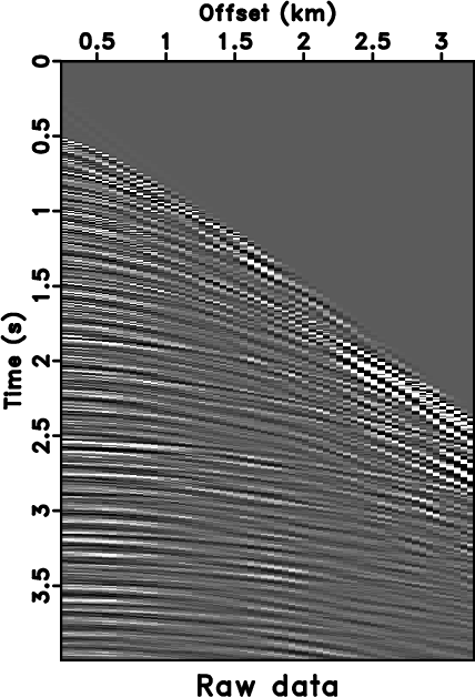
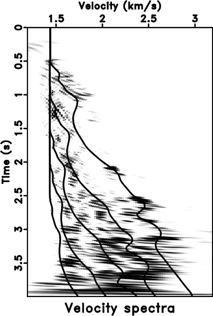
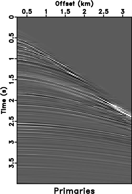
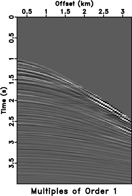
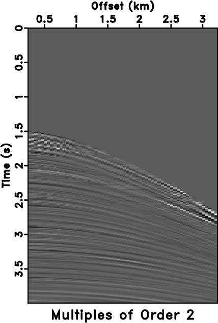
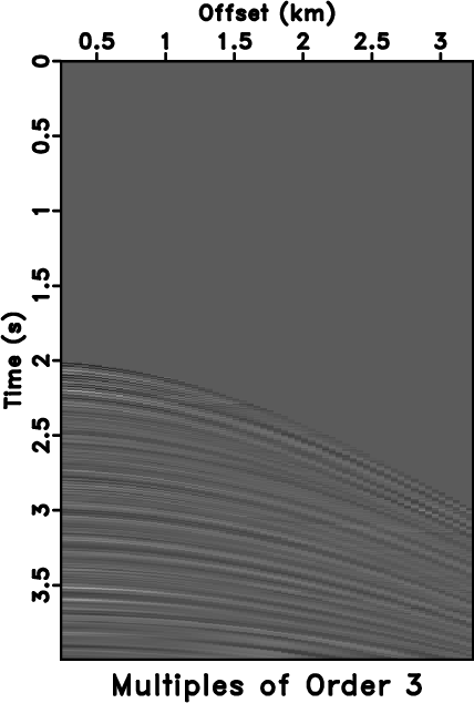
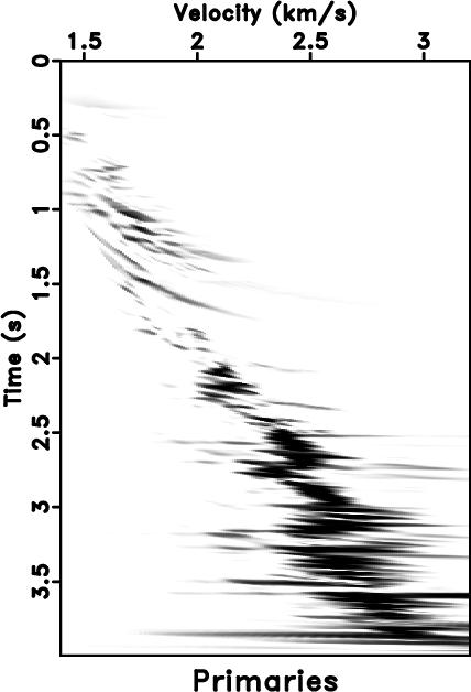
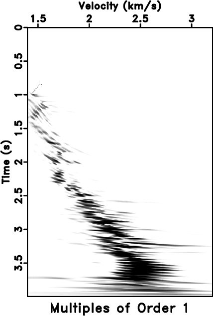
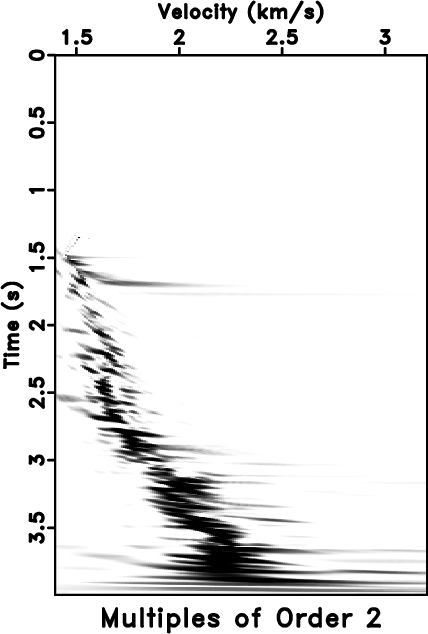
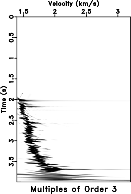
Next, we test the proposed algorithm to separate multi-wavefields on a single CMP gather from the Viking Graben (Mobil AVO) dataset (Keys and Foster, 1998). The field data are shown in Figure 10a. We pick the primary velocities by muting spectra energy of multiples. Multiple RMS velocities with different orders (equation 9) follow the pseudo-primary NMO equation 8. The velocity spectra of primaries and multiples are shown in Figure 10b. Equations 7 and 10 convert velocities to slopes, which help the VD-seislet frame separate primaries from different-order pegleg multiples (we only display three orders). Figure 11 displays the separated primaries and different-order multiples. The corresponding velocity spectra are shown in Figure 12. After separating different wavefields, the velocity spectra confirm that the signals get concentrated around their respective trends.
|
|---|
|
cmp,rvscan
Figure 10. Field CMP gather (a) and velocity trends of primaries and multiples (b). |
|
|
|
|---|
|
rcomp0,rcomp1,rcomp2,rcomp3
Figure 11. Separated wavefields. Primaries (a), first-order multiples (b), second-order multiples (c), and third-order multiples (d). |
|
|
|
|---|
|
rvscan0,rvscan1,rvscan2,rvscan3
Figure 12. Velocity spectra of different wavefields. Primaries (a), first-order multiples (b), second-order multiples (c), and third-order multiples (d). |
|
|
|
|
|
|
Signal and noise separation in prestack seismic data using velocity-dependent seislet transform |