Wavefield extrapolation in pseudodepth domain

Vertical time coordinate frame

The concept of vertical time has a long history in seismic exploration. Vertical time $\tau$ is the vertical axis for time migration (Yilmaz, 2001; Claerbout, 1985). It is defined as the two-way traveltime measured by coinciding source and receiver on the surface

$$\tau_{TW}(z) = 2 \int_0^z \frac{\mathrm{d} z^\prime}{v(z^\prime)} .$$ (1)

For conventional time image applications, this equation is used in the context of laterally invariant media. This is however, not adequate for imaging complex strudtures. We argue that vertical time, although does not correspond to the actual two-way traveltime in complex velocites, still works fine as representation of the vertical axis. Since wavefield extrapolation is usually not zero-offset, in this work we will use the one-way vertical time, defined as

$$\tau(x,y,z) = \int_0^z \frac{\mathrm{d} z^\prime}{v_m(x,y,z^\prime)} ,$$ (2)

Note that velocity $v_m$ does not have to be identical to the velocity in which we propagate wavefields. For example, one can choose a constant $v_m$ , then the vertical time is simply a scaled version of depth, $\tau = z / v_m$ . In practice, we suggest using a smooth background velocity as $v_m$ , because it helps regularize $\tau$ coordinate grids. Here we retain the name ``vertical time'' for $\tau$ , however, it should not be confused with the vertical time $\tau_{TW}$ used in time processing. In other words, Equation 2 represent only a change of variable from $z$ to $\tau$ .

Normally, wavefields are discretized on the Cartesian mesh with equally-spaced grids. For a monochromatic wave, wavelength changes with velocity and since the grid spacing is held constant, the number of samples per wavelength increases in layers with high velocities and decreases in layers with low velocities. To avoid spatial aliasing, the maximum grid spacing is limited by $\Delta x \leq v_{\min} / (2 f_{\max})$ , where $v_{\min}$ is the lowest velocity, often located in shallow layers. As a result, the deep layers with high velocities are often oversampled. The increased sampling of the layers with high velocity raises the cost of wavefield extrapolation without enhancing image resolution. Introducing vertical time partially resolves this problem. This can be seen by taking difference of equation 2 between to time levels,

$$\Delta\tau \equiv \tau_{n+1} - \tau_{n} = \int_{z(\tau_n)}^{z(\tau_{n+1})} \frac{\mathrm{d} z^\prime}{v_m(x,y,z^\prime)} ,$$ (3)

which corresponds to a fixed $\tau$ sampling, $\Delta\tau$ . This implies that the effective sampling in depth $z(\tau_{n+1}) - z(\tau_n)$ increases with velocity.

uCT Figure 1. wavelength variation with depth $z$ (Left) and vertical time $\tau$ (Right) of a $5$ Hz sine. The velocity profile is $v=1500+0.7z \; \mathrm{m/sec}$ .

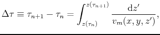
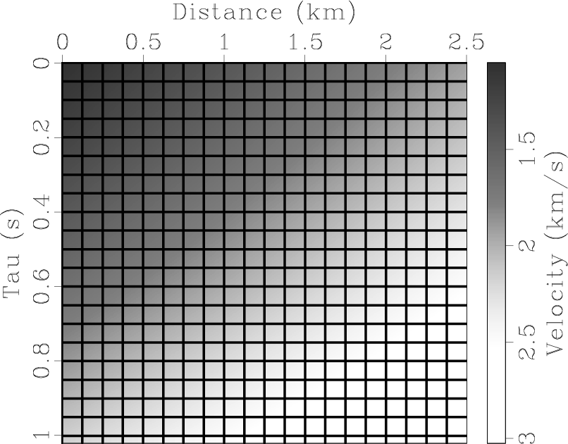
Figure 1 shows a comparison of vertical sampling in depth $z$ and vertical time $\tau$ . In the Cartesian domain on the left, the sampling of the wavefield is relatively coarse in shallow layers and becomes finer with depth. In the $\tau$ domain on the right, the wavefield is evenly sampled in spite of the velocity variation, for the same number of samples.

Equation 2 maps a depth point $(x,y,z)$ to vertical time point $(x,y,\tau)$ . The inverse mapping is also straighforward, from differentiation of inverse functions, it follows

$$z(x,y,\tau) = \int_0^\tau v_m(x,y,\tau^\prime) \mathrm{d} \tau^\prime ,$$ (4)

where the integration constant is zero because $\tau(z=0)=0$ .

By changing the vertical axis from $z$ to $\tau$ , the coordinate system is effectively changed from the Cartesian frame $\lbrace x_1,x_2,x_3\rbrace$ to a new coordinate frame $\lbrace\xi_1,\xi_2,\xi_3\rbrace$ , where the two coordinate systems are related by

$$\xi_1 = x_1 \quad, \xi_2 = x_2 \quad, \xi_3 = \tau = \int_0^{x_3} \frac{\mathrm{d} x_3^\prime}{v_m(x_1,x_2,x_3^\prime)}$$ (5)

As long as the funtions $x_i(\xi_1,\xi_2,\xi_3)$ and $\xi_i(x_1,x_2,x_3)$ are one-to-one and free from singularities, we can interpolate any space functions between the Cartesian and $\tau$ domains. Figures 2(a) to 3(b) illustrate examples of such interpolations. The velocity field in the $\tau$ domain is obtained by interpolating the velocity in the Cartesian domain using Equation 2. In Figures 2(a) and 2(b), the mapping velocity $v_m$ is computed by stacking the true velocity $v$ horizontally, and thus it is laterally constant. As a result, the $\tau$ coordinate system is orthogonal. In Figures 3(a) and 3(b), $\tau$ is computed from the true velocity, i.e. $v_m=v$ , the resulting $\tau$ coordinate system is nonorthogonal due to the lateral variation of $v$ .

linA,linB
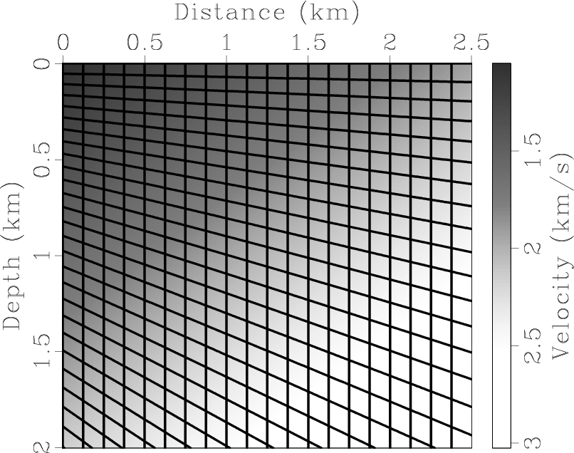
Figure 2. A linear velocity model in (a) Cartesian domain and (b) orthogonal $\tau$ domain overlaid with $\tau$ domain mesh. The velocity is $v=1250+0.35x+0.3z \; \mathrm{m/sec}$ .

linC,linD
Figure 3. The same velocity model as in Figure 2(a) in (a) Cartesian domain and (b) nonorthogonal $\tau$ domain overlaid with $\tau$ domain mesh.

The new coordinate system $(x,y,\tau)$ has mixed units of time in the vertical axis and distance in the horizontal axes. Sometime it is more convenient to have distance units in all three axes of the space domain. To achieve this we can simply scale $\tau$ by some velocity funciton $\tilde{v}$

$$\tilde{z}(\tau) = \int_0^\tau \tilde{v}(\tau^\prime) \mathrm{d} \tau^\prime = \int_0^z \frac{\tilde{v}}{v_m} \mathrm{d} z^\prime$$ (6)

For example, if $\tilde{v}$ is set to constant, the pseudodepth is simply a linear scaling of $\tau$ , $\tilde{z}(\tau) = \tilde{v} \tau$ . The importance of this step will be evident later as we look into anisotropic media.

Wavefield extrapolation in pseudodepth domain