|
|
|
|
Solving 3D Anisotropic Elastic Wave Equations on Parallel GPU Devices |
In this section we demonstrate the utility of the GPU-based modeling approach by presenting reproducible numerical tests using the 2D/3D elastic FDTD codes for different TI models. The first set of tests involve applying the FDTD code to 2D homogeneous isotropic and VTI media. We define our test isotropic medium by P- and S-wave velocities of ![]() =2.0 km/s and
=2.0 km/s and ![]() =
=
![]() , and a density of
, and a density of ![]() =2000 kg/m
=2000 kg/m![]() . The VTI medium uses the same
. The VTI medium uses the same ![]() ,
, ![]() and
and ![]() , but includes three Thomsen parameters (Thomsen, 1986) of
, but includes three Thomsen parameters (Thomsen, 1986) of
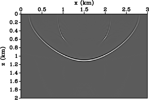
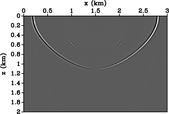
![]() . Figures 5(a)-(b) present the vertical and horizontal components,
. Figures 5(a)-(b) present the vertical and horizontal components, ![]() and
and ![]() respectively, of the 2D isotropic impulse response tests, while Figures 5(c)-(d) show the similar components for the VTI model. Both tests generate the expected wavefield responses when compared to the CPU-only code results.
respectively, of the 2D isotropic impulse response tests, while Figures 5(c)-(d) show the similar components for the VTI model. Both tests generate the expected wavefield responses when compared to the CPU-only code results.


|
|---|
|
ISO-UZ,ISO-UX,VTI-UZ,VTI-UX
Figure 5. 2D Impulse response tests with the ewefd2d_gpu modelling code. (a) Isotropic model |
|
|
Figure 6 presents comparative GPU versus CPU metrics for a number of squared (![]() ) model domains and runs of 1000 time steps. We ran the OpenMP-enabled CPU ewefd2d code on a dedicated workstation with a dual quad-core Intel Xeon chipset, and computed the corresponding GPU benchmarks on the 480-core NVIDIA GTX 480 GPU card. Because we output receiver data at every tenth time step, the reported runtimes involve both parallel and serial sections, which hides some of the speedup advantage of the GPU parallelism. Figure 6(a) presents computational runtimes for the CPU (red line) and GPU (blue line) implementations. The reported runtime numbers are the mean value of ten repeat trials conducted for each data point. Figure 6(b) shows the 10
) model domains and runs of 1000 time steps. We ran the OpenMP-enabled CPU ewefd2d code on a dedicated workstation with a dual quad-core Intel Xeon chipset, and computed the corresponding GPU benchmarks on the 480-core NVIDIA GTX 480 GPU card. Because we output receiver data at every tenth time step, the reported runtimes involve both parallel and serial sections, which hides some of the speedup advantage of the GPU parallelism. Figure 6(a) presents computational runtimes for the CPU (red line) and GPU (blue line) implementations. The reported runtime numbers are the mean value of ten repeat trials conducted for each data point. Figure 6(b) shows the 10![]() speedup of the GPU implementation relative the CPU-only version.
speedup of the GPU implementation relative the CPU-only version.


|
|---|
|
Runtimes,Speedup
Figure 6. GPU (blue line) versus CPU (red line) performance metrics showing the mean of ten trials for various square ( |
|
|
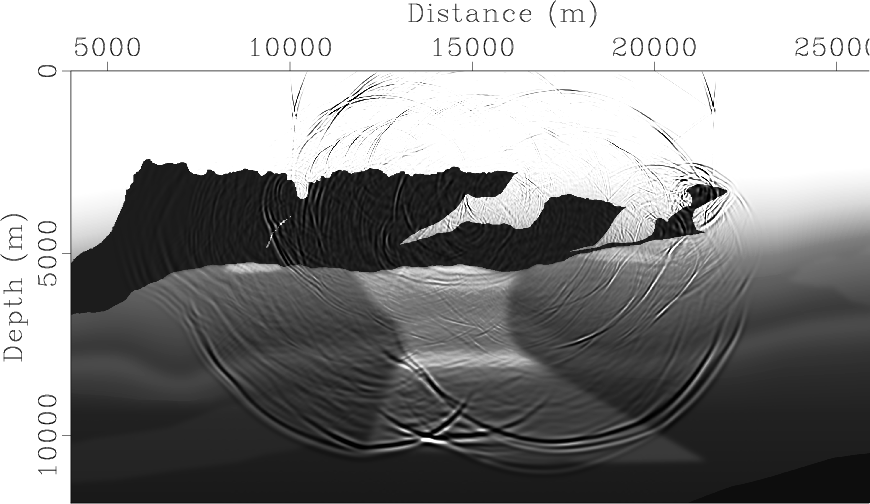
Our second example tests the relative accuracy of the two implementations on a heterogenous isotropic elastic model. We use the publicly available P-wave velocity and density models of the 2004 BP synthetic dataset (Billette and Brandsberg-Dahl, 2005), and assume a S-wave model defined by
![]() . We use temporal and spatial sampling intervals of
. We use temporal and spatial sampling intervals of
![]() ms and
ms and
![]() km and inject a 40 Hz Ricker wavelet as a stress source for each wavefield component.
km and inject a 40 Hz Ricker wavelet as a stress source for each wavefield component.
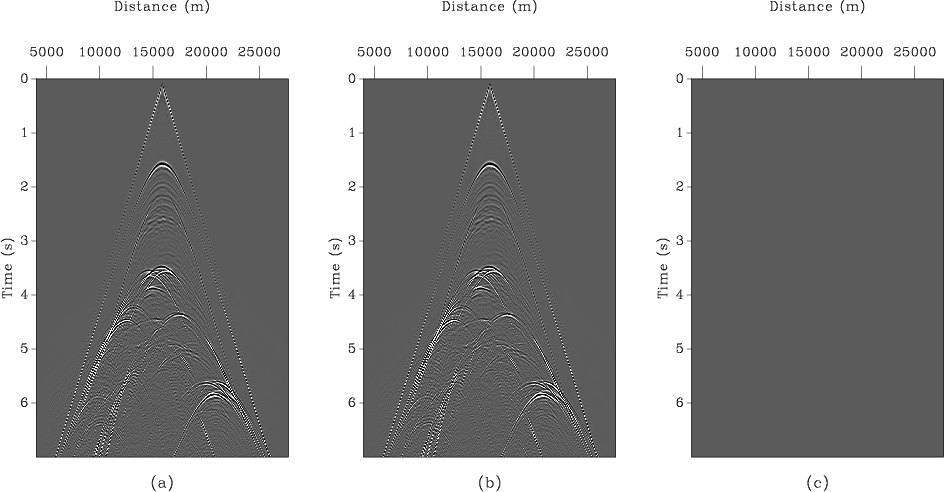
Figure 7 shows a snapshot of the propagating wavefield overlying the P-wave velocity model. Figures 8(a)-(b) presents the corresponding data from the CPU and GPU implementations, respectively, while Figure 8(c) shows their difference clipped to the same scale. The ![]() energy norm in the difference panel is roughly
energy norm in the difference panel is roughly
![]() of that in the CPU/GPU versions, indicating that the GPU version is accurate to within a modest amount above floating-point precision. This slight discrepancy is expected due to the differences in treatment of math operations between the GPU and CPU hardware (Whitehead and Fit-Florea, 2011); however, we assert that this will not create problems for realistic modeling applications.
of that in the CPU/GPU versions, indicating that the GPU version is accurate to within a modest amount above floating-point precision. This slight discrepancy is expected due to the differences in treatment of math operations between the GPU and CPU hardware (Whitehead and Fit-Florea, 2011); however, we assert that this will not create problems for realistic modeling applications.
|
|---|
|
wavevel
Figure 7. Wavefield snapshot overlying part of the P-wave model of the realistic BP velocity synthetic. |
|
|
|
|---|
|
BPdata
Figure 8. Data Modeled through for BP velocity synthetic model. (a) GPU implementation. (b) CPU implementation. (c) Data difference between GPU and CPU implementations clipped at the same level as (a) and (b). |
|
|
|
|
|
|
Solving 3D Anisotropic Elastic Wave Equations on Parallel GPU Devices |