|
|
|
|
Wavefield extrapolation in pseudodepth domain |
Using the ![]() domain two-way wave equation 15, we apply reverse-time migration to Sigsbee2a synthetic dataset.
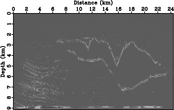
Figure 10(a) shows a standard RTM image obtained in the Cartesian domain. The vertical axis, depth
domain two-way wave equation 15, we apply reverse-time migration to Sigsbee2a synthetic dataset.
Figure 10(a) shows a standard RTM image obtained in the Cartesian domain. The vertical axis, depth ![]() , is discretized into
, is discretized into ![]() samples.
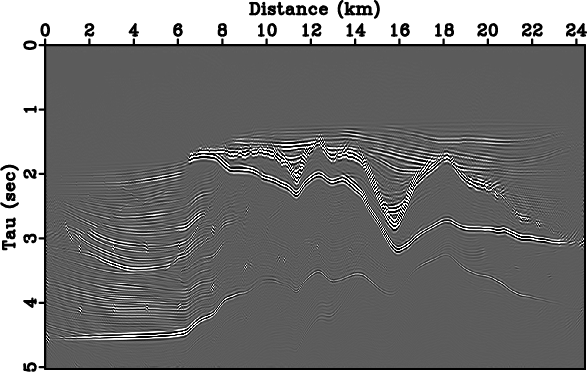
Figure 10(b) shows an RTM image obtained in
samples.
Figure 10(b) shows an RTM image obtained in ![]() domain. The vertical axis has been replaced by vertical time
domain. The vertical axis has been replaced by vertical time ![]() , with
, with ![]() samples.
Thus, the model size in the
samples.
Thus, the model size in the ![]() domain has been reduced by
domain has been reduced by ![]() compared to the Cartesian domain.
Measured by wall clock times, the
compared to the Cartesian domain.
Measured by wall clock times, the ![]() domain RTM gained a total of
domain RTM gained a total of ![]() speedup compared to Cartesian domain RTM, which as expected, is close to the reduction of the model size.
speedup compared to Cartesian domain RTM, which as expected, is close to the reduction of the model size.

|
|---|
|
sigsC,sigsT,sigsB
Figure 10. Prestack migration of the Sigsbee dataset. Images are obtained in (a) Cartesian and (b) |
|
|
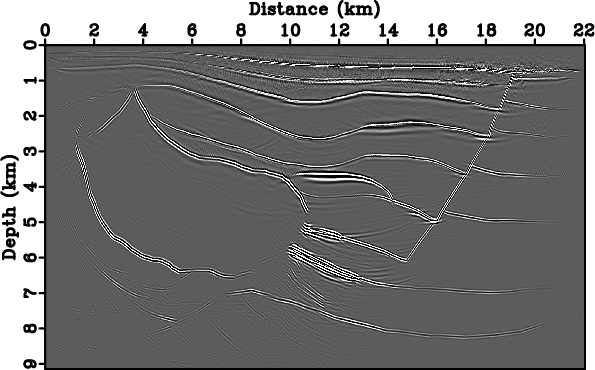
Similarly, anisotropic reverse-time migration can be implemented using Equation 21.
Figure 11(a) illustrates a migrated image of the SEG/Hess salt dataset, with ![]() samples in vertical direction. In the
samples in vertical direction. In the ![]() domain, the models are discretized into
domain, the models are discretized into ![]() samples in vertical direction.
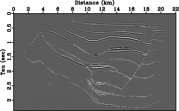
Figure 11(b) illustrates the
samples in vertical direction.
Figure 11(b) illustrates the ![]() domain migration image. Again, the
domain migration image. Again, the ![]() domain RTM has seen
domain RTM has seen ![]() speedup, due to a corresponding sampling reduction of
speedup, due to a corresponding sampling reduction of ![]() . Note as well that the first two reflections in the
. Note as well that the first two reflections in the ![]() domain result is not aliased compared to its depth counterpart. This implies that if these reflections are crucial, then we will require even a denser depth sampling to avoid aliasing
up shallow. This will result in even a larger cost difference.
domain result is not aliased compared to its depth counterpart. This implies that if these reflections are crucial, then we will require even a denser depth sampling to avoid aliasing
up shallow. This will result in even a larger cost difference.

|
|---|
|
hessC,hessT,hessB
Figure 11. Prestack migration of the SEG/Hess dataset. Images are obtained in (a) Cartesian and (b) |
|
|
|
|
|
|
Wavefield extrapolation in pseudodepth domain |