A fast butterfly algorithm for generalized Radon transforms

Acknowledgments

We are grateful to Tariq Alkhalifah, Anatoly Baumstein, Ian Moore, Daniel Trad, and the anonymous reviewer for their valuable comments and suggestions. We thank Dr. Alexander Klokov for preprocessing the field data. We thank KAUST and sponsors of the Texas Consortium for Computational Seismology (TCCS) for financial support.

Appendix A

The mathematical derivation of the fast butterfly algorithm

This appendix gives a complete derivation and description of the butterfly algorithm, which combines the low-rank approximations and the butterfly structure introduced in the main text. For more mathematical exposition, the reader is referred to Candès et al. (2009).

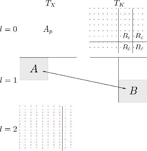
To facilitate the presentation, we add a new figure (Figure A-1) to illustrate the notations.

1. Initialization. At level $l=0$ , let $A$ be the root box of $T_X$ . For each leaf box $B\in T_K$ , expressions 9 and 10 are valid as $w(B)\leq 1/\sqrt{N}$ . Substituting $\beta_t^{AB}$ (in equation 10) into the definition of $\delta_t^{AB}$ , equation 21, we get

$$\delta_t^{AB}=e^{-2\pi i \Phi(\mathbf{x}_0(A),\mathbf{k}_t^B)}\su... ...B(\mathbf{k}) e^{2\pi i \Phi(\mathbf{x}_0(A),\mathbf{k})}g(\mathbf{k}) \right),$$ (32)

i.e. the equation 23 in the main text. In addition, for $\mathbf{x}\in A$ , the partial sum $u^B(\mathbf{x})$ in equation 20 is given by (with $\alpha_t^{AB}$ (in equation 9) plugged in)

$$u^{B}(\mathbf{x}) \approx \sum_t e^{2\pi i \Phi(\mathbf{x},\mathbf{k}_t^B)}\delta_t^{AB}.$$ (33)

Comparing the right hand sides of equations 19 and A-2, if we call $g(\mathbf {k})$ the sources at $\mathbf {k}$ , then coefficients $\delta_t^{AB}$ are just like the equivalent sources at $\mathbf{k}_t^B$ . This initial step is to redistribute the original sources $g(\mathbf {k})$ located at $\mathbf {k}$ (denoted by blue dots in Figure A-1) to equivalent sources $\delta^{AB}_t$ located at Chebyshev grid $\mathbf{k}_t^B$ (not shown in the figure). We next aim at updating $\delta_t^{AB}$ until the end level $L$ .

2. Recursion. At $l=1,2,...,L/2$ , for each pair $(A,B)$ , let $A_p$ be $A$ 's parent and $\{B_c, c=1,2,3,4\}$ be $B$ 's children from the previous level (see Figure A-1). For each child $B_c$ , we have available from the previous level an approximation of the form

$$u^{B_c}(\mathbf{x})\approx \sum_{t'} e^{2\pi i \Phi(\mathbf{x},\mathbf{k}_{t'}^{B_c})}\delta_{t'}^{A_pB_c}, \ \ \mathbf{x}\in A_p.$$ (34)

Summing over all children gives

$$u^{B}(\mathbf{x})\approx \sum_c \sum_{t'} e^{2\pi i \Phi(\mathbf{x},\mathbf{k}_{t'}^{B_c})}\delta_{t'}^{A_pB_c}, \ \ \mathbf{x}\in A_p.$$ (35)

Since $A\subset A_p$ , this is of course true for any $\mathbf{x}\in A$ . Also we know that equation 17 holds for $\mathbf{k}_{t'}^{B_c}\in B$ , i.e.,

$$e^{2\pi \Phi(\mathbf{x},\mathbf{k}_{t'}^{B_c})}\approx\sum_t e^{2\pi i \Phi(\mathbf{x},\mathbf{k}_t^B)}\beta_t^{AB}(\mathbf{k}_{t'}^{B_c}), \ \ \mathbf{x}\in A.$$ (36)

Inserting it into expression A-4 yields

$$u^{B}(\mathbf{x})\approx \sum_c \sum_{t'} \sum_t e^{2\pi i \Phi(\mathbf{x},\mathbf{k}_t^B)}\beta_t^{AB}(\mathbf{k}_{t'}^{B_c})\delta_{t'}^{A_pB_c}, \ \ \mathbf{x}\in A.$$ (37)

On the other hand, $u^B(\mathbf{x})$ admits a low-rank approximation of equivalent sources at the current level,

$$u^{B}(\mathbf{x})\approx \sum_t e^{2\pi i \Phi(\mathbf{x},\mathbf{k}_{t}^{B})}\delta_{t}^{AB}, \ \ \mathbf{x}\in A.$$ (38)

Equating expressions A-6 and A-7 suggests that we can take

$$\delta_t^{AB}=\sum_c\sum_{t'}\beta_t^{AB}(\mathbf{k}_{t'}^{B_c})\delta_{t'}^{A_pB_c}.$$ (39)

Substituting $\beta_t^{AB}$ (in equation 10), we get

$$\delta_t^{AB}=e^{-2\pi i \Phi(\mathbf{x}_0(A),\mathbf{k}_t^B)}\su... ...2\pi i \Phi(\mathbf{x}_0(A),\mathbf{k}_{t'}^{B_c})}\delta_{t'}^{A_pB_c}\right),$$ (40)

i.e. the equation 24 in the main text.

3. Switch. A switch of the representation to expressions 11 and 12 is needed at the middle level $l=L/2$ since expressions 9 and 10 are no longer valid as soon as $l>L/2$ (boxes $B$ are getting bigger and bigger so that $w(B)\leq 1/\sqrt{N}$ is no longer satisfied). Plugging $\beta_t^{AB}$ (in equation 12) into the definition of $\delta_t^{AB}$ , equation 21, one has

$$\delta_t^{AB}=\sum_{\mathbf{k}\in B}e^{2\pi \Phi(\mathbf{x}_t^A,\mathbf{k})}g(\mathbf{k})=u^B(\mathbf{x}_t^A);$$ (41)

from expression A-7,

$$u^B(\mathbf{x}_t^A)\approx \sum_s e^{2\pi i \Phi(\mathbf{x}_t^A,\mathbf{k}_s^B)}\delta_s^{AB},$$ (42)

where we use $\{\delta_t^{AB}\}$ to denote the new set of coefficients and $\{\delta_s^{AB}\}$ the old set. Equating expressions A-10 and A-11, we can set $\delta_t^{AB}$ as

$$\delta^{AB}_t= \sum_s e^{2\pi i \Phi(\mathbf{x}_t^A,\mathbf{k}_s^B)}\delta_s^{AB},$$ (43)

i.e. the equation 25 in the main text. This middle step is to switch from equivalent sources $\delta_s^{AB}$ located at Chebyshev grid $\mathbf{k}_s^B$ on the $K$ side to equivalent sources $\delta_t^{AB}$ located at Chebyshev grid $\mathbf{x}_t^A$ on the $X$ side.

4. Recursion. The rest of the recursion is analogous to Step 2. For $l=L/2+1,...,L$ , we have

$$u^{B}(\mathbf{x})\approx \sum_c \sum_{t'} \alpha_{t'}^{A_pB_c}(\mathbf{x})\delta_{t'}^{A_pB_c}, \ \ \mathbf{x}\in A_p,$$ (44)

thus

$$u^{B}(\mathbf{x}_t^A)\approx \sum_c \sum_{t'} \alpha_{t'}^{A_pB_c}(\mathbf{x}_t^A)\delta_{t'}^{A_pB_c};$$ (45)

recalling expression A-10, one can simply set

$$\delta_t^{AB}=\sum_c \sum_{t'} \alpha_{t'}^{A_pB_c}(\mathbf{x}_t^A)\delta_{t'}^{A_pB_c}.$$ (46)

Inserting $\alpha_t^{AB}$ (in equation 11) gives the update

$$\delta_t^{AB}=\sum_c e^{2\pi i \Phi(\mathbf{x}_t^A,\mathbf{k}_0(B... ...pi i \Phi(\mathbf{x}_{t'}^{A_p},\mathbf{k}_0(B_c))}\delta_{t'}^{A_pB_c}\right),$$ (47)

i.e. the equation 26 in the main text.

5. Termination. Finally we reach the level $l=L$ , and $B$ is the entire domain $K$ . For every box $A$ in $X$ and every $\mathbf{x}\in A$ ,

$$u(\mathbf{x})=u^{B}(\mathbf{x})\approx \sum_t \alpha_t^{AB}(\mathbf{x})\delta_t^{AB}.$$ (48)

Plugging in $\alpha_t^{AB}$ (in equation 11), we get

$$u(\mathbf{x})=e^{2\pi i \Phi(\mathbf{x},\mathbf{k}_0(B))}\sum_t \... ...thbf{x}) e^{-2\pi i \Phi(\mathbf{x}_t^A,\mathbf{k}_0(B))} \delta_t^{AB}\right),$$ (49)

i.e. the equation 27 in the main text. This final step is to transform the equivalent sources $\delta_t^{AB}$ located at Chebyshev grid $\mathbf{x}_t^A$ back to the targets $u(\mathbf {x})$ located at $\mathbf {x}$ (denoted by red dots in Figure A-1).

In the above algorithm, $L=\log N$ is assumed to be an even number. If $L$ is odd, one can either switch at level $(L-1)/2$ or $(L+1)/2$ . Everything else remains unchanged.

illus
Figure A-1. The butterfly structure for the special case of $N=4$ . The top right panel represents the input domain $K$ with sources $g(\mathbf {k})$ located at $\mathbf {k}$ (blue dots). The bottom left panel represents the output domain $X$ with targets $u(\mathbf {x})$ located at $\mathbf {x}$ (red dots). For the pair of boxes $(A,B)$ at level $l=1$ , box $A_p$ is called $A$ 's parent at the previous level; four small boxes $B_c$ are called $B$ 's children at the previous level.

A fast butterfly algorithm for generalized Radon transforms